人工智能实战第5次作业_许骏鹏

人工智能第五次作业

一、作业要求

项目	内容
这个作业属于哪个课程	人工智能实战
这个作业的要求在哪里	click_here
我在这个课程的目标是	获得实战经验
这个作业在哪个具体方面帮助我实现目标	学会用sigmoid激活函数来实现二分类

二、代码实现

import numpy as np
import matplotlib.pyplot as plt


def Read_AND_Data():
    X = np.array([0, 0, 1, 1, 0, 1, 0, 1]).reshape(2, 4)
    Y = np.array([0, 0, 0, 1]).reshape(1, 4)
    return X, Y


def Read_OR_Data():
    X = np.array([0, 0, 1, 1, 0, 1, 0, 1]).reshape(2, 4)
    Y = np.array([0, 1, 1, 1]).reshape(1, 4)
    return X, Y


def Sigmoid(x):
    s = 1 / (1 + np.exp(-x))
    return s


# 前向计算
def ForwardCalculationBatch(W, B, batch_X):
    Z = np.dot(W, batch_X) + B
    A = Sigmoid(Z)
    return A


# 反向传播
def BackPropagationBatch(batch_X, batch_Y, A):
    m = batch_X.shape[1]
    dZ = A - batch_Y
    dB = dZ.sum(axis=1, keepdims=True) / m
    dW = np.dot(dZ, batch_X.T) / m
    return dW, dB


# 参数更新
def UpdateWeights(W, B, dW, dB, eta):
    W = W - eta * dW
    B = B - eta * dB
    return W, B


# 计算损失函数
def CheckLoss(W, B, X, Y):
    m = X.shape[1]
    A = ForwardCalculationBatch(W, B, X)
    J = np.sum(-(np.multiply(Y, np.log(A)) + np.multiply(1 - Y, np.log(1 - A))))
    loss = J / m
    return loss


# 初始化参数
def InitialWeights(num_input, num_output):
    W = np.zeros((num_output, num_input))
    B = np.zeros((num_output, 1))
    return W, B


# 训练
def train(X, Y, ForwardCalculationBatch, CheckLoss):
    num_example = X.shape[1]  # 4
    num_feature = X.shape[0]  # 2
    num_category = Y.shape[0]  # 1
    # hyper parameters
    eta = 0.5
    max_epoch = 10000
    # W(num_category, num_feature), B(num_category, 1)
    W, B = InitialWeights(num_feature, num_category)
    # calculate loss to decide the stop condition
    loss = 5  # initialize loss (larger than 0)
    error = 2e-3  # stop condition
    # if num_example=200, batch_size=10, then iteration=200/10=20
    for epoch in range(max_epoch):
        for i in range(num_example):
            # get x and y value for one sample
            x = X[:, i].reshape(num_feature, 1)
            y = Y[:, i].reshape(1, 1)
            # get z from x,y
            batch_a = ForwardCalculationBatch(W, B, x)
            # calculate gradient of w and b
            dW, dB = BackPropagationBatch(x, y, batch_a)
            # update w,b
            W, B = UpdateWeights(W, B, dW, dB, eta)
            # end if
        # end for
        # calculate loss for this batch
        loss = CheckLoss(W, B, X, Y)
        print(epoch, i, loss, W, B)
        # end if
        if loss < error:
            break
            # end for
    return W, B, epoch, loss

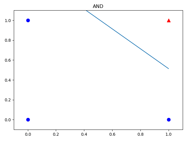
# 结果可视化
def ShowResult(W,B,X,Y,title):
    # 根据w, b的值画出分割线
    w = -W[0,0]/W[0,1]
    b = -B[0,0]/W[0,1]
    x = np.array([0,1])
    y = w * x + b
    plt.plot(x,y)
    # 画出原始样本值
    for i in range(X.shape[1]):
        if Y[0,i] == 0:
            plt.scatter(X[0,i],X[1,i],marker="o",c='b',s=64)
        else:
            plt.scatter(X[0,i],X[1,i],marker="^",c='r',s=64)
    plt.axis([-0.1,1.1,-0.1,1.1])
    plt.title(title)
    plt.show()

if __name__ == '__main__':
    X, Y = Read_AND_Data()
    W, B, epoch, loss = train(X, Y, ForwardCalculationBatch, CheckLoss)
    ShowResult(W,B,X,Y,"AND")
    

三、结果展示