计算机视觉学习7_多视图几何_基础矩阵

对极几何

多视图几何是利用在不同视点所拍摄图像间的关系，来研究照相机之间或者特征之间关系的一门科学。
图像的特征通常是兴趣点。
多视图几何中最重要的内容是双视图几何。

对极点 = 基线与像平面相交点 = 光心在另一幅图像中的投影
对极平面 = 包含基线的平面
对极线 = 对极平面与像平面的交线

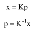
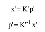
本质矩阵（Essentical Matrix）

本质矩阵描述了空间中的点在两个世界坐标系中的坐标对应关系

若相机内参矩阵K已知，则可以从空间点坐标推算出图像点坐标


则根据三线共面，有

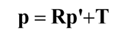
（T×p）得到是垂直于平面的向量

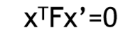
基本矩阵（Fundamental Matrix）

基础矩阵是对极几何的代数表达方式
本质矩阵描述了空间中的点在两个图像的投影的对应关系
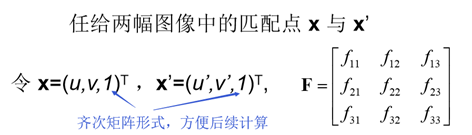
（图像中任意对应点 x↔x’ 之间的约束关系）

F 为 3x3 矩阵，秩为2，对任意匹配点对 x↔x’ 均满足

8点算法估算基础矩阵F

基础矩阵FF是一个3×3的矩阵，有9个未知元素。然而，上面的公式中使用的齐次坐标，齐次坐标在相差一个常数因子下是相等，F也就只有8个未知元素，也就是说，只需要8对匹配的点对就可以求解出两视图的基础矩阵FF。下面介绍下8点法 Eight-Point-Algorithm计算基础矩阵的过程。

则：

A·x=0
A·AT -> 最小特征值，对应特征向量

上述求解后的F不一定能满足秩为2的约束，因此 还要在F基础上加以约束。

矩阵各列的数据尺度差异太大，会导致部分 元素被忽略
——> 最小二乘得到的结果精度一般很低

归一化8点算法

归一化8点算法将图像坐标范围限定在 ~[-1,1]x[1,1]，实验表明可以得到更可靠的结果。

实现代码

from PIL import Image
from numpy import *
from pylab import *
import numpy as np
from PCV.geometry import camera
from PCV.geometry import homography
from PCV.geometry import sfm
from PCV.localdescriptors import sift


# Read features
# 载入图像，并计算特征
im1 = array(Image.open('../mydata/test1.jpg'))
sift.process_image('../mydata/test1.jpg', 'im1.sift')
l1, d1 = sift.read_features_from_file('im1.sift')

im2 = array(Image.open('../mydata/test2.jpg'))
sift.process_image('../mydata/test2.jpg', 'im2.sift')
l2, d2 = sift.read_features_from_file('im2.sift')

# 匹配特征
matches = sift.match_twosided(d1, d2)
ndx = matches.nonzero()[0]

# 使用齐次坐标表示，并使用 inv(K) 归一化
x1 = homography.make_homog(l1[ndx, :2].T)
ndx2 = [int(matches[i]) for i in ndx]
x2 = homography.make_homog(l2[ndx2, :2].T)

x1n = x1.copy()
x2n = x2.copy()
print(len(ndx))

figure(figsize=(16,16))
sift.plot_matches(im1, im2, l1, l2, matches, True)
show()

# Don't use K1, and K2

#def F_from_ransac(x1, x2, model, maxiter=5000, match_threshold=1e-6):
def F_from_ransac(x1, x2, model, maxiter=5000, match_threshold=1e-6):
    """ Robust estimation of a fundamental matrix F from point
    correspondences using RANSAC (ransac.py from
    http://www.scipy.org/Cookbook/RANSAC).

    input: x1, x2 (3*n arrays) points in hom. coordinates. """

    from PCV.geometry import ransac
    data = np.vstack((x1, x2))
    d = 20 # 20 is the original
    # compute F and return with inlier index
    F, ransac_data = ransac.ransac(data.T, model,
                                   8, maxiter, match_threshold, d, return_all=True)
    return F, ransac_data['inliers']

# find E through RANSAC
# 使用 RANSAC 方法估计 E
model = sfm.RansacModel()
F, inliers = F_from_ransac(x1n, x2n, model, maxiter=5000, match_threshold=1e-4)

print(len(x1n[0]))
print(len(inliers))

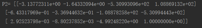
# 计算照相机矩阵（P2 是 4 个解的列表）
P1 = array([[1, 0, 0, 0], [0, 1, 0, 0], [0, 0, 1, 0]])
P2 = sfm.compute_P_from_fundamental(F)

# triangulate inliers and remove points not in front of both cameras
X = sfm.triangulate(x1n[:, inliers], x2n[:, inliers], P1, P2)

# plot the projection of X
cam1 = camera.Camera(P1)
cam2 = camera.Camera(P2)
x1p = cam1.project(X)
x2p = cam2.project(X)

figure()
imshow(im1)
gray()
plot(x1p[0], x1p[1], 'o')
#plot(x1[0], x1[1], 'r.')
axis('off')

figure()
imshow(im2)
gray()
plot(x2p[0], x2p[1], 'o')
#plot(x2[0], x2[1], 'r.')
axis('off')
show()

figure(figsize=(16, 16))
im3 = sift.appendimages(im1, im2)
im3 = vstack((im3, im3))

imshow(im3)

cols1 = im1.shape[1]
rows1 = im1.shape[0]
for i in range(len(x1p[0])):
    if (0<= x1p[0][i]<cols1) and (0<= x2p[0][i]<cols1) and (0<=x1p[1][i]<rows1) and (0<=x2p[1][i]<rows1):
        plot([x1p[0][i], x2p[0][i]+cols1],[x1p[1][i], x2p[1][i]],'c')
axis('off')
show()

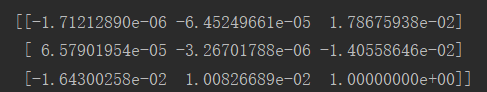
print(F)



x1e = []
x2e = []
ers = []
for i,m in enumerate(matches):
    if m>0: #plot([locs1[i][0],locs2[m][0]+cols1],[locs1[i][1],locs2[m][1]],'c')
        x1=int(l1[i][0])
        y1=int(l1[i][1])
        x2=int(l2[int(m)][0])
        y2=int(l2[int(m)][1])
        # p1 = array([l1[i][0], l1[i][1], 1])
        # p2 = array([l2[m][0], l2[m][1], 1])
        p1 = array([x1, y1, 1])
        p2 = array([x2, y2, 1])
        # Use Sampson distance as error
        Fx1 = dot(F, p1)
        Fx2 = dot(F, p2)
        denom = Fx1[0]**2 + Fx1[1]**2 + Fx2[0]**2 + Fx2[1]**2
        e = (dot(p1.T, dot(F, p2)))**2 / denom
        x1e.append([p1[0], p1[1]])
        x2e.append([p2[0], p2[1]])
        ers.append(e)
x1e = array(x1e)
x2e = array(x2e)
ers = array(ers)

indices = np.argsort(ers)
x1s = x1e[indices]
x2s = x2e[indices]
ers = ers[indices]
x1s = x1s[:20]
x2s = x2s[:20]

figure(figsize=(16, 16))
im3 = sift.appendimages(im1, im2)
im3 = vstack((im3, im3))

imshow(im3)

cols1 = im1.shape[1]
rows1 = im1.shape[0]
for i in range(len(x1s)):
    if (0<= x1s[i][0]<cols1) and (0<= x2s[i][0]<cols1) and (0<=x1s[i][1]<rows1) and (0<=x2s[i][1]<rows1):
        plot([x1s[i][0], x2s[i][0]+cols1],[x1s[i][1], x2s[i][1]],'c')
axis('off')
show()

实现结果

室外图像对（一张近拍，一张远拍）

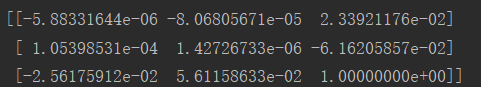
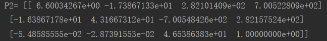
基础矩阵F:

相机矩阵（投影矩阵）：

sift特征匹配

蓝色为投影特征点，红色为原始特征点

室内图像对

基础矩阵：

相机矩阵（投影矩阵）：

三维重建

from PIL import Image
from numpy import *
from pylab import *
import numpy as np
from PCV.geometry import camera
from PCV.geometry import homography
from PCV.geometry import sfm
from PCV.localdescriptors import sift
# 标定矩阵
K = array([[2394,0,932],[0,2398,628],[0,0,1]])
# 载入图像，并计算特征


im1 = array(Image.open('../mydata/j1.jpg'))
sift.process_image('../mydata/j1.jpg','im1.sift')
l1,d1 = sift.read_features_from_file('im1.sift')

im2 = array(Image.open('../mydata/j2.jpg'))
sift.process_image('../mydata/j2.jpg','im2.sift')
l2,d2 = sift.read_features_from_file('im2.sift')

# 匹配特征
matches = sift.match_twosided(d1,d2)
ndx = matches.nonzero()[0]

# 使用齐次坐标表示，并使用 inv(K) 归一化
x1 = homography.make_homog(l1[ndx,:2].T)
ndx2 = [int(matches[i]) for i in ndx]
x2 = homography.make_homog(l2[ndx2,:2].T)
x1n = dot(inv(K),x1)
x2n = dot(inv(K),x2)

# 使用 RANSAC 方法估计 E
model = sfm.RansacModel()
E,inliers = sfm.F_from_ransac(x1n,x2n,model)
# 计算照相机矩阵（P2 是 4 个解的列表）
P1 = array([[1,0,0,0],[0,1,0,0],[0,0,1,0]])
P2 = sfm.compute_P_from_essential(E)

# 选取点在照相机前的解
ind = 0
maxres = 0
for i in range(4):
    # 三角剖分正确点，并计算每个照相机的深度
    X = sfm.triangulate(x1n[:,inliers],x2n[:,inliers],P1,P2[i])
    d1 = dot(P1,X)[2]
    d2 = dot(P2[i],X)[2]

    if sum(d1>0)+sum(d2>0) > maxres:
        maxres = sum(d1>0)+sum(d2>0)
        ind = i
        infront = (d1>0) & (d2>0)
    # 三角剖分正确点，并移除不在所有照相机前面的点
    X = sfm.triangulate(x1n[:,inliers],x2n[:,inliers],P1,P2[ind])
    X = X[:,infront]

    # 绘制三维图像
    from mpl_toolkits.mplot3d import axes3d
    fig = figure()
    ax = fig.gca(projection='3d')
    ax.plot(-X[0], X[1], X[2], 'k.')
    axis('off')
    # 绘制 X 的投影 import camera
    # 绘制三维点
    cam1 = camera.Camera(P1)
    cam2 = camera.Camera(P2[ind])
    x1p = cam1.project(X)
    x2p = cam2.project(X)

    # 反 K 归一化
    x1p = dot(K, x1p)
    x2p = dot(K, x2p)
    figure()
    imshow(im1)
    gray()
    plot(x1p[0], x1p[1], 'o')
    plot(x1[0], x1[1], 'r.')
    axis('off')
    figure()
    imshow(im2)
    gray()
    plot(x2p[0], x2p[1], 'o')
    plot(x2[0], x2[1], 'r.')
    axis('off')
    show()

PS:
报错：

原因：匹配的点过少
解决
1、重拍一对照片
2、改大阈值
F, inliers = F_from_ransac(x1n, x2n, model, maxiter=5000, match_threshold=1e-4)
改为
F, inliers = F_from_ransac(x1n, x2n, model, maxiter=5000, match_threshold=3)