A Mathematical Introduction to Robotic Manipulation - 2 (part 3)

版权声明：本文为博主原创文章，未经博主允许不得转载。 https://blog.csdn.net/mobius_strip/article/details/89357827

4 Velocity of a Rigid Body

In this section, we derive a formula for the velocity of a rigid body whose motion is given by $g(t)$, a curve parameterized by time t in $SE(3)$. This is not such a naive question as in the case of a single particle following a curve $q(t) ∈ \mathbb R^3$, where the velocity of the particle is $v_q(t) = \frac{d}{dt}q(t)$, because this notion of velocity cannot be generalized since $SE(3)$ is not Euclidean. In particular, the quantity $\dot g(t) \not\in SE(3)$ and $\dot g(t) \not\in se(3)$ and the question of its connection with rotational and translational velocity needs to be handled with care. Further, the definition of velocity needs to relate to our informal understanding of rotational and translational velocity. We will show that the proper representation of rigid body velocity is through the use of twists.

4.1 Rotational velocity

Consider first the case of pure rotational motion in $\mathbb R^3$. Let $R_{ab}(t) ∈ SO(3)$ be a curve representing a trajectory of an object frame B, with origin at the origin of frame A, but rotating relative to the fixed frame A. We call A the spatial coordinate frame and B the body coordinate frame. Any point q attached to the rigid body follows a path in spatial coordinates given by

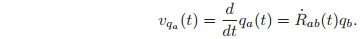
Note that the coordinates$ q_b$ are fixed in the body frame. The velocity of the point in spatial coordinates is

Thus R˙ ab maps the body coordinates of a point to the spatial velocity of that point. This representation of the rotational velocity is somewhat inefficient, since it requires nine numbers to describe the velocity of a rotating body. One may use the special structure in the matrix $\dot R_{ab}$ to derive a more compact representation. To this end, we rewrite equation as

The following lemma shows that $\dot R_{ab}(t)R_{ab}^{−1}(t) ∈ so(3)$; i.e., it is skew-symmetric.

Lemma 2.12. Given $R(t) ∈ SO(3)$, the matrices $\dot R(t)R^{−1}(t) ∈ \mathbb R^{3×3}$ and $R^{−1}(t)\dot R(t) ∈ \mathbb R^{3×3}$ are skew-symmetric.

Lemma 2.12 allows us to represent the velocity of a rotating body using a 3-vector. We define the instantaneous spatial angular velocity, denoted $ω^s_{ab} ∈ \mathbb R^3$, as

The vector $ω^s_{ab}$ corresponds to the instantaneous angular velocity of the object as seen from the spatial (A) coordinate frame. Similarly, we define the instantaneous body angular velocity, denoted $ω_{ab}^b ∈ \mathbb R^3$, as

The body angular velocity describes the angular velocity as viewed from the instantaneous body (B) coordinate frame. From these two equations, it follows that the relationship between the two angular velocities is

We can express the velocity of a point in terms of the instantaneous angular velocity of the rigid body


Above two equations constitute a compact description of the velocity of all particles of the body in terms of the body and spatial angular velocities, $ω_{ab}^b$ and $ω_{ab}^s$.

4.2 Rigid body velocity

Let us now consider the general case where $g_{ab}(t) ∈ SE(3)$ is a one-parameter curve (parameterized by time) representing a trajectory of a rigid body: more specifically, the rigid body motion of the frame B attached to the body, relative to a fixed or inertial frame A. As in the case of rotation, $\dot g_{ab}(t)$ by itself is not particularly useful, but the two terms $\dot g_{ab}g_{ab}^{−1}$ and $g_{ab}^{−1} \dot g_{ab}$ have some special significance. With

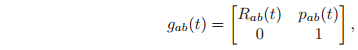
we have that

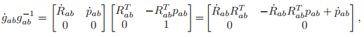
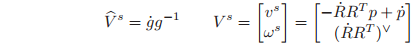
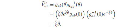
which has the form of a twist. By analogy to the rotational velocity, we define the spatial velocity $\hat V_{ab}^s ∈ se(3)$ as

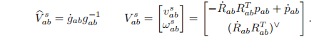
The spatial velocity $\hat V_{ab}^s$ can be used to find the velocity of a point in spatial coordinates. The coordinates of a point q attached to the rigid body in spatial coordinates are given by

Differentiating yields

and thus,

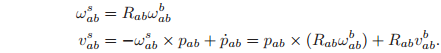
The interpretation of the components of the spatial velocity of a rigid motion is somewhat unintuitive. The angular component, $ω_{ab}^s$, is the instantaneous angular velocity of the body as viewed in the spatial frame. The linear component, vab s , is not the velocity of the origin of the body frame, which is apparent from equation (2.53). Rather, $v_{ab}^s(t)$ is the velocity of a (possibly imaginary) point on the rigid body which is traveling through the origin of the spatial frame at time $t$. That is, if one stands at the origin of the spatial frame and measures the instantaneous velocity of a point attached to the rigid body and traveling through the origin at that instant, this is $v_{ab}^s(t)$.

A somewhat more natural interpretation of the spatial velocity is obtained by using the relationship between twists and screws described in the previous section. The screw associated with the twist $\hat V_{ab}^s$ gives the instantaneous axis, pitch, and magnitude of the rigid motion relative to the spatial frame.

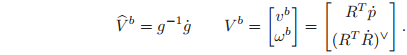
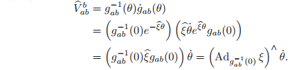
It is also possible to specify the velocity of a rigid body with respect to the (instantaneous) body frame. We define

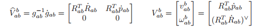
to be the body velocity of a rigid motion $g_{ab}(t) ∈ SE(3)$. The velocity of the point in the body frame is given by

Thus, the action of $\hat V_{ab}^b$ is to take the body coordinates of a point, $q_b$, and return the velocity of that point written in body coordinates, $v_{q_b}$:

The interpretation of the body velocity is straightforward: $v_{ab}^b$ is the velocity of the origin of the body coordinate frame relative to the spatial frame, as viewed in the current body frame. ωab b is the angular velocity of the coordinate frame, also as viewed in the current body frame. Note that the body velocity is not the velocity of the body relative to the body frame; this latter quantity is always zero.

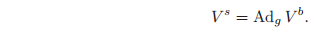
The spatial and body velocity of a rigid motion are related by a similarity transformation. To calculate this relationship, we note that

Alternatively, we can write

In either case, we may summarize the calculation as

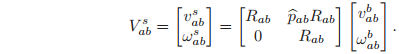
The 6 × 6 matrix which transforms twists from one coordinate frame to another is referred to as the adjoint transformation associated with $g$, written $Ad_g$. Thus, given $g ∈ SE(3)$ which maps one coordinate system into another, $Ad_g : \mathbb R^6 → \mathbb R^6$ is given as

In the calculation that we have just performed, $Ad_g$ maps body velocity twist coordinates to spatial velocity twist coordinates. $Ad_g$ is invertible, and its inverse is given by

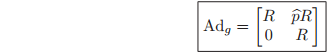
We shall make frequent use of the adjoint transformations throughout the book. The calculations performed above give the following useful characterization of the adjoint associated with a rigid transformation $g ∈ SE(3)$:

Lemma 2.13. If $\hat ξ∈ se(3)$ is a twist with twist coordinates $ξ ∈ \mathbb R^6$, then for any $g ∈ SE(3), g\hat ξg^{−1}$ is a twist with twist coordinates $Ad_g ξ ∈ \mathbb R^6$.

It will often be convenient to define velocity without explicit reference to coordinate frames. For a rigid body with configuration $g ∈ SE(3)$, we define the spatial velocity as

and the body velocity as

The body and spatial velocities are related by the adjoint transformation,

4.3 Velocity of a screw motion

Consider the more general case where

represents the configuration of coordinate frame B relative to frame A. Using the fact that for a constant twist $\hat ξ$,

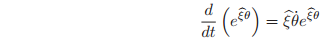
the spatial velocity for this rigid body motion is

Thus, the spatial velocity corresponding to this motion is precisely the velocity generated by the screw.

The body velocity of a screw motion can be calculated in a similar manner:

4.4 Coordinate transformations

Just as we can compose rigid body transformations to find $g_{ac} ∈ SE(3)$ given $g_{ab}, g_{bc} ∈ SE(3)$, it is possible to determine the velocity of one coordinate frame relative to a third given the relative velocities between the first and second and second and third coordinate frames. We state the main results as a set of propositions.

Proposition 2.14. Transformation of spatial velocities
Consider the motion of three coordinate frames, A, B, and C. The following relation exists between their spatial velocities:

Proposition 2.15. Transformation of body velocities
Consider motion of three coordinate frames, A, B, and C. The following relation exists between their relative body velocities:

A few other identities between body and spatial velocities will prove useful in subsequent chapters. We give them here in the form of a lemma.
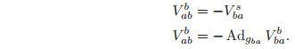
Lemma 2.16. Rigid body velocity identities
Using the notation given above for the velocity of one coordinate frame relative to another, the following relationships hold:

5 Wrenches and Reciprocal Screws

5.1 Wrenches

A generalized force acting on a rigid body consists of a linear component (pure force) and an angular component (pure moment) acting at a point. We can represent this generalized force as a vector in $\mathbb R^6$:

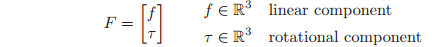
We will refer to a force/moment pair as a wrench.

The values of the wrench vector $F ∈ \mathbb R^6$ depend on the coordinate frame in which the force and moment are represented. If B is a coordinate frame attached to a rigid body, then we write $F_b = (f_b,τ_b)$ for a wrench applied at the origin of B, with $f_b$ and $τ_b$ specified with respect to the B coordinate frame.

Wrenches combine naturally with twists to define instantaneous work. Consider the motion of a rigid body parameterized by $g_{ab}(t)#, where A is an inertial frame and B is a frame attached to the rigid body. Let $V^b_{ab} ∈ \mathbb R^6$ represent the instantaneous body velocity of the rigid body and let $F_b$ represent an applied wrench. Both of these quantities are represented relative to the B coordinate frame and their dot product is the infinitesimal work:

The net work generated by applying the wrench $F_b$ through a twist $V_{ab}^b$ over a time interval $[t_1,t_2]$ is given by


Two wrenches are said to be equivalent if they generate the same work for every possible rigid body motion. Equivalent wrenches can be used to rewrite a given wrench in terms of a wrench applied at a different point (and with respect to a different coordinate frame). An example of this is shown in Figure 2.13: given the wrench Fb applied at the origin of contact coordinate frame B, we wish to determine the equivalent wrench applied at the origin of the object coordinate frame C. In order to compute the equivalent wrench, we use the instantaneous work performed by the wrench as the body undergoes an arbitrary rigid motion. Let $g_{bc} = (p_{bc},R_{bc})$ be the configuration of frame C relative to B. By equating the instantaneous work done by the wrench Fb and the wrench Fc over an arbitrary interval of time, we have that

and since $V^b_{ac}$ is free,

Equation transforms a wrench applied at the origin of the B frame into an equivalent wrench applied at the origin of the C frame. The components of $F_c$ are specified relative to the C coordinate frame. Expanding equation,

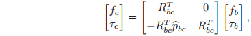
we see that the adjoint transformation rotates the force and torque vectors from the B frame into the C frame and includes an additional torque of the form $−p_{bc} × f_b$, which is the torque generated by applying a force $f_b$ at a distance $−p_{bc}$.

It is also possible to represent a wrench with respect to a coordinate frame which is not inside the rigid body. Consider for example the coordinate frame A shown in Figure 2.13. The wrench F written in A’s coordinate frame is given by

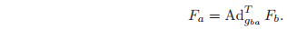
This wrench represents the equivalent force/moment pair applied as if the coordinate frame A were rigidly attached to the object. This is not the same as simply rewriting the components of $F_b$ in A’s coordinates, since the point of application for Fa is the origin of the A frame and not the origin of the B frame.

If several wrenches are all applied to a single rigid body, then the net wrench acting on the rigid body can be constructed by adding the wrench vectors. In order for this addition to make sense, all of the wrenches must be represented with respect to the same frame. Thus, given a set of wrenches $F_i$, each wrench is first written as an equivalent wrench relative to a single coordinate frame and then the equivalent wrenches are added to determine the net wrench acting on the rigid body. This helps explain why equivalent wrenches include a shift of origin: one can only add wrenches if they represent forces and torques applied at a single point (such as the center of mass or a fixed spatial frame).

A net wrench F acting on a rigid body with configuration $g_{ab} ∈ SE(3)$ has two natural representations. The body representation of the wrench is written as $F_b$ and represents the equivalent force and moment applied at the origin of the B frame (and written in B’s coordinates). The spatial representation of the wrench is the equivalent wrench written in A’s coordinate frame. These representations are analogous to the spatial and body representations of the velocity of a rigid body.

As with velocities, it will be convenient to define the spatial and body representations of a wrench without explicit reference to a given set of coordinate frames. If $g ∈ SE(3)$ is the configuration of a rigid body, then we write F b for the body wrench and $F_s$ for the spatial wrench. These wrenches are related by the transpose of the adjoint matrix:

This notation mirrors that used for body and spatial velocities of a rigid body allowing the instantaneous work performed by a wrench $F$ moving through a rigid motion with instantaneous velocity $V$ to be written as

5.2 Screw coordinates for a wrench

As with twists, it is possible to generate a wrench by applying a force along an axis in space and simultaneously applying a torque about the same axis. The dual of Chasles’ theorem, which showed that every twist could be generated by a screw, is called Poinsot’s theorem. It asserts that every wrench is equivalent to a force and torque applied along the same axis. We begin by defining the notion of a wrench acting along a screw.
With respect to some fixed spatial coordinate frame A, let $S$ be a screw with axis $l = {q + λω : λ ∈ R}, \Vert ω \Vert = 1$, pitch $h$, and magnitude $M$. We construct a wrench from this screw by applying a force of magnitude $M$ along the directed line $l$ and a torque of magnitude $hM$ about the line. If $h = ∞$, we generate a wrench by applying a pure torque about $l$. The resulting wrench, in A’s coordinates, is given by

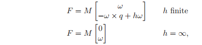
where the term $−ω × q$ accounts for the offset between the axis of the screw and the origin of A. We call F the wrench along the screw $S$. Note that $F$ (and $q$ and $ω$) are all specified with respect to the fixed coordinate frame A and hence $F$ represents the spatial wrench applied to the rigid body. (We omit the use of subscripts in this section since all quantities are specified with respect to a single coordinate frame.)

To find the screw coordinates for a wrench, we solve equation for $ω, q, h$, and $M$ given $F = (f, τ)$. This leads to the following theorem:

Theorem 2.17 (Poinsot). Every collection of wrenches applied to a rigid body is equivalent to a force applied along a fixed axis plus a torque about the same axis.

Using Poinsot’s theorem, we can define the screw coordinates of a wrench, $F = (f, τ)$:

1. Pitch:
   
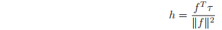
   The pitch of a wrench is the ratio of angular torque to linear force. If $f = 0$, we say that $F$ has infinite pitch.
2. Axis:
   
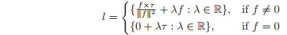
   The axis $l$ is a directed line through a point. For $f \neq 0$, the axis is a line in the f direction going through the point $q = frac{f×τ}{\Vert f \Vert^2}$. For $f = 0$, the axis is a line in the $τ$ direction going through the origin.
3. Magnitude:
   
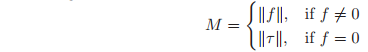
   The magnitude of a screw is the net linear force, if the motion contains a linear component, or the net torque, otherwise.

The dual nature of twists and wrenches is evident in the screw coordinates for twists and wrenches. For example, a zero pitch twist corresponds to pure rotation, while a zero pitch wrench corresponds to a pure force (no angular component).

5.3 Reciprocal screws

The dot product between twists and wrenches gives the instantaneous power associated with moving a rigid body through an applied force. As in the previous subsection, we carry out all calculations relative to a single coordinate frame and omit the use of subscripts. A wrench $F$ is said to be reciprocal to a twist $V$ if the instantaneous power is zero: $F · V = 0$. Since both twists and wrenches can be represented by screws, we can use this to define the notion of reciprocal screws:

Definition 2.3. Reciprocal screws
Two screws $S_1$ and $S_2$ are reciprocal if the twist $V$ about $S_1$ and the wrench $F$ along $S_2$ are reciprocal.

Classically, reciprocal screws are defined by using the reciprocal product between screws. Let $S_i$ be a screw with axis $l_i = {q_i + λω_i : λ ∈ R}$, pitch $h_i$, and magnitude $M_i$. Given two screws $S_1$ and $S_2$, we define the distance $d$ between the screws as the minimum distance between $l_1$ and $l_2$; this distance will be achieved along a line perpendicular to both $l_1$ and $l_2$. We denote this line as $d_n$ where $n$ is a unit vector and $d > 0$. The angle $α$ between $S_1$ and $S_2$ is the angle between the vectors $ω_1$ and $ω_2$,

(see Figure 2.15). The reciprocal product between two screws is defined as

Proposition 2.18. Characterization of reciprocal screws
Two screws $S_1$ and $S_2$ are reciprocal if and only if

If we represent screws using twist coordinates, then we can define the reciprocal product directly in terms of the components of the twists. Let $V_1, V_2 ∈ \mathbb R^6$ be two arbitrary twists. Then we define the reciprocal product between $V_1$ and $V_2$ as

A similar relationship holds if we associate screws with wrenches.

If we interpret a set of screws ${S_1,... ,S_k}$ as twists, then the twists form a linear space over the reals and hence we can talk about scaling and adding screws by interpreting this in terms of regular addition and multiplication on twists. We call the set of screws ${S_1,... ,S_k}$ a system of screws and we define addition and scaling of screws by associating each screw with a unique twist.

It follows immediately from the definition of the reciprocal product that if $S$ is reciprocal to $S_1$ and $S_2$, then it is reciprocal to any linear combination of $S_1$ and $S_2$ (with the linear combination performed in twist coordinates). Using this linearity property, we can define the set of all screws which are reciprocal to a given system of screws as the reciprocal screw system. A reciprocal screw system defines a linear subspace of twists. If we interpret a screw system as a set of wrenches (or constrained directions), then the reciprocal screw system describes the instantaneous motions which are possible under the constraints. Conversely, if we interpret the screw system as a set of twists, then the reciprocal screw system is the set of wrenches which cause no net motion of the object. Both of these interpretations follow directly from the definition of the reciprocal product between a twist and a wrench.

Proposition 2.19. Dimensionality of reciprocal screw systems
Let r be the dimension of system of screws ${S_1, . . . , S_k}$ (determined by converting the screws into either twists or wrenches) and let $n$ be the dimension of the corresponding reciprocal system. Then,

6 Summary

The following are the key concepts covered in this chapter:

reference

A Mathematical Introduction to Robotic Manipulation Richard M. Murray, Zexiang Li, S. Shankar Sastry