3 Rigid Motion in
Recall from Section 1 that a rigid motion is one that preserves the distance between points and the angle between vectors.
In general, rigid motions consist of rotation and translation. The procedure for representing pure translational motion is very simple: choose a (any) point in the body and keep track of the coordinates of the point relative to some known frame. This gives a curve , for a trajectory of the entire rigid body.
The representation of general rigid body motion, involving both translation and rotation, is more involved. We describe the position and orientation of a coordinate frame B attached to the body relative to an inertial frame A (see Figure 2.3). Let
be the position vector of the origin of frame B from the origin of frame A, and
the orientation of frame B, relative to frame A. A configuration of the system consists of the pair
, and the configuration space of the system is the product space of
with
, which shall be denoted as
(for special Euclidean group):

As in the case of
, there is a generalization to
dimensions,

Analogous to the rotational case, an element
serves as both a specification of the configuration of a rigid body and a transformation taking the coordinates of a point from one frame to another. More precisely, let
be the coordinates of a point q relative to frames A and B, respectively. Given
, we can find qa by a transformation of coordinates:

where
is the specification of the configuration of
the B frame relative to the A frame. By an abuse of notation, we write
to denote the action of a rigid transformation on a point,

so that
.
The action of a rigid transformation
on a vector
is defined by the following formula:

Thus, a vector is transformed by rotation.
3.1 Homogeneous representation
The transformation of points and vectors by rigid transformations has a simple representation in terms of matrices and vectors in
. We begin by adopting some notation. We append 1 to the coordinates of a point to yield a vector in
,
These are called the homogeneous coordinates of the point q. Thus, the origin has the form
Vectors, which are the difference of points, then have the form
Note that the form of the vector is different from that of a point. The 0 and 1 in the fourth component of vectors and points, respectively, will remind us of the difference between points and vectors and enforce a few rules of syntax:
- Sums and differences of vectors are vectors.
- The sum of a vector and a point is a point.
- The difference between two points is a vector.
- The sum of two points is meaningless.
The transformation
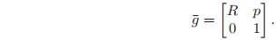
given in equation is an affine transformation. Using the preceding notation for points, we may represent it in linear form by writing it as
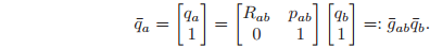
The 4 × 4 matrix
is called the homogeneous representation of
. In general, if
, then
The price to be paid for the convenience of having a homogeneous or linear representation of the rigid body motion is the increase in the dimension of the quantities involved from 3 to 4.
The last row of the matrix of equation appears to be “extra baggage” as well. However, in the graphics literature, the number 1 is frequently replaced by a scalar constant which is either greater than 1to represent dilation or less than 1 to represent contraction. Also, the row vector of zeros in the last row may be replaced by some other row vector to provide “perspective transformations.” In both these instances, of course, the transformation represented by the augmented matrix no longer corresponds to a rigid displacement.
Rigid body transformations can be composed to form new rigid body transformations. Let
be the configuration of a frame C relative to a frame B, and gab the configuration of frame B relative to another frame A. Then, using equation, the configuration of C relative to frame A is given by
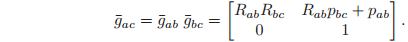
Equation defines the composition rule for rigid body transformations to be the standard matrix multiplication. Using the homogeneous representation, it may be verified that the set of rigid transformations is a group; that is:
- If , then .
- The 4 × 4 identity element, , is in .
- If
, then the inverse of
is determined by straightforward
matrix inversion to be:
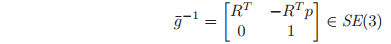
so that . - The composition rule for rigid body transformations is associative.
Using the homogeneous representation for a vector , we obtain the representation for a rigid body transformation of by multiplying the homogeneous representations of by the homogeneous representation of ,
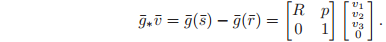
Note that by defining the homogeneous representation of a vector to have a zero in the bottom row, we are able to once again use matrix multiplication to represent the action of a rigid transformation, this time on a vector instead of a point. For notational simplicity, in what follows we will confuse homogeneous representations and the abstract representation of points, vectors, and rigid body transformations. Thus, we will write
and
instead of
and
.
The next proposition establishes that elements of are indeed rigid body transformations; namely, that they preserve angles between vectors and distances between points.
Proposition 2.7. Elements of SE(3) represent rigid motions
Any
is a rigid body transformation:
-
preserves distance between points:

-
preserves orientation between vectors:

Proof. The proofs follow directly from the corresponding proofs for rotation matrices:

3.2 Exponential coordinates for rigid motion and twists
The notion of the exponential mapping introduced in Section 2 for
can be generalized to the Euclidean group,
. We will make extensive use of this representation in the sequel since it allows an elegant, rigorous, and geometric treatment of spatial rigid body motion. We begin by presenting a pair of motivational examples and then present a formal set of definitions.

Consider the simple example of a one-link robot as shown in Figure 2.5a, where the axis of rotation is
, and
is a point on the axis. Assuming that the link rotates with unit velocity, then the velocity of the tip point,
, is

This equation can be conveniently converted into homogeneous coordinates by defining the 4 × 4 matrix
to be
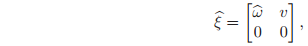
with
. Equation can then be rewritten with an extra row appended to it as
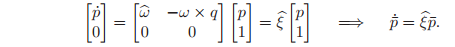
The solution of the differential equation is given by

where
b is the matrix exponential of the 4 × 4 matrix
, defined (as usual) by
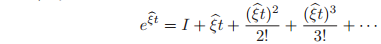
The scalar t is the total amount of rotation (since we are rotating with unit velocity). exp(
) is a mapping from the initial location of a point to its location after rotating t radians.
In a similar manner, we can represent the transformation due to translational motion as the exponential of a 4 × 4 matrix. The velocity of a point attached to a prismatic joint moving with unit velocity (see Figure 2.5b) is

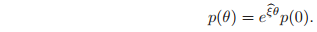
Again, the solution of equation (2.27) can be written as exp(
)p(0)$, where t is the total amount of translation and
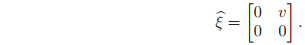
The 4 × 4 matrix given in equations is the generalization of the skew-symmetric matrix . Analogous to the definition of , we define

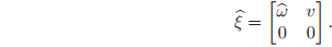
In homogeneous coordinates, we write an element
as
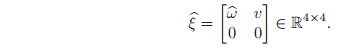
An element of
is referred to as a twist, or a (infinitesimal) generator of the Euclidean group. We define the ∨ (vee) operator to extract the 6-dimensional vector which parameterizes a twist,
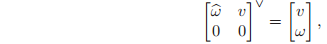
and call
the twist coordinates of
. The inverse operator, ∧ (wedge), forms a matrix in
out of a given vector in
:
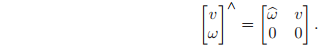
Thus,
represents the twist coordinates for the twist
; this parallels our notation for skew-symmetric matrices.
Proposition 2.8. Exponential map from
to
Given
and
, the exponential of
is an element of
, i.e.,

Proof. The proof is by explicit calculation. In the course of the proof, we will obtain a formula for exp(
). Write
as
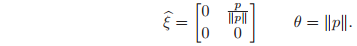
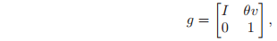
Case 1
. If
, then a straightforward calculation shows that

so that exp(
)
and hence
which is in
as desired.
Case 2
. Assume
, by appropriate scaling of
if necessary, and define a rigid transformation
by
Now, using the calculation of Lemma 2.3, with
, we have
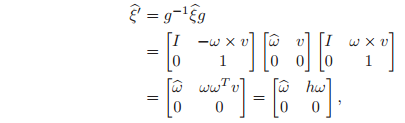
where
. Using the following identity,

it suffices to calculate exp(
). This simplifies the calculation since it may be verified (using
) that

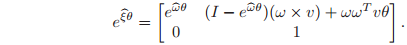
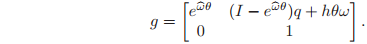
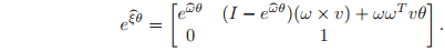
Hence,
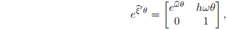
and using equation it follows that
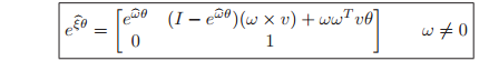
which is an element of
.
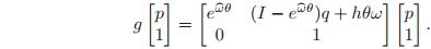
The transformation
\hat ξθ$) is slightly different than the rigid transformations that we have encountered previously. We interpret it not as mapping points from one coordinate frame to another, but rather as mapping points from their initial coordinates,
, to their coordinates after the rigid motion is applied:
In this equation, both
and
are specified with respect to a single reference frame. Similarly, if we let
represent the initial configuration of a rigid body relative to a frame A, then the final configuration, still with respect to A, is given by

Thus, the exponential map for a twist gives the relative motion of a rigid body.
Proposition 2.9. Surjectivity of the exponential map onto
Given
, there exists
and
such that
exp(
.
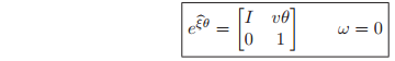
Case 1 (
). If there is no rotational motion, set
Equation verifies that exp
.
Case 2 (
). To find
, we equate exp
and g and solve
for
. Using equation:
and
are obtained by solving the rotation equation exp
, as in Proposition 2.5 of the previous section. This leaves the equation

which must be solved for v. It suffices to show that the matrix

is nonsingular for all
. This follows from the fact that the two matrices which comprise A have mutually orthogonal null spaces when
(and
). Hence,
.
In light of Proposition 2.9, every rigid transformation g can be written as the exponential of some twist . We call the vector the exponential coordinates for the rigid transformation g. Note that, as in the case of rotations, the mapping exp : is many-to-one since the choice of and for solving the rotational component of the motion is not unique. This does not present great difficulties since for most applications we are given the twist as part of the problem and we wish to find the corresponding rigid motion.
3.3 Screws: a geometric description of twists
In this section, we explore some of the geometric attributes associated with a twist
. These attributes give additional insight into the use of twists to parameterize rigid body motions. We begin by defining a specific class of rigid body motions, called screw motions, and then show that a twist is naturally associated with a screw.

Consider a rigid body motion which consists of rotation about an axis in space through an angle of θ radians, followed by translation along the same axis by an amount d as shown in Figure 2.7a. We call such a motion a screw motion, since it is reminiscent of the motion of a screw, in so far as a screw rotates and translates about the same axis. To further encourage this analogy, we define the pitch of the screw to be the ratio of translation to rotation,
(assuming
). Thus, the net translational motion after rotating by
radians is
. We represent the axis as a directed line through a point; choosing
to be a point on the axis and
to be a unit vector specifying the direction, the axis is the set of points

The above definitions hold when the screw motion consists of a nonzero rotation followed by translation.
In the case of zero rotation, the axis of the screw must be defined differently: we take the axis as the line through the origin in the direction v (i.e., v is a vector of magnitude 1), as shown in Figure 2.7b. By convention, the pitch of this screw is and the magnitude is the amount of translation along the direction v. Collecting these, we have the following definition of a screw:
Definition 2.2. Screw motion
A screw
consists of an axis
, a pitch
, and a magnitude
. A screw motion represents rotation by an amount
about the axis l followed by translation by an amount
parallel to the axis l. If
then the corresponding screw motion consists of a pure translation along the axis of the screw by a distance
.

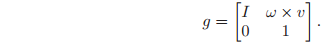
To compute the rigid body transformation associated with a screw, we analyze the motion of a point
, as shown in Figure 2.8. The final location of the point is given by

or, in homogeneous coordinates,
Since this relationship must hold for all
, the rigid motion given by the screw is
As in the last section, this transformation maps points attached to the rigid body from their initial coordinates (
) to their final coordinates, and all points are specified with respect to the fixed reference frame.
Note that the rigid body displacement given in equation (2.40) has the same form as the exponential of a twist, given in equation (2.36):
In fact, if we choose
(only when
is orthogonal to
, this is true), then
generates the screw motion in equation (2.40) (assuming
). In the case of a pure rotation,
and the twist associated with a screw motion is simply
. In the instance that the screw corresponds to pure translation, we let θ be the amount of translation, and the rigid body motion described by this “screw” is
which is precisely the motion generated by exp(
) with
. Thus, we see that a screw motion corresponds to motion along a constant twist by an amount equal to the magnitude of the screw.
In fact, we can go one step further and define a screw associated with every twist. Let be a twist with twist coordinates . We do not assume that , allowing both translation plus rotation as well as pure translation. The following are the screw coordinates of a twist:
- Pitch
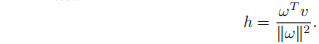
- Axis:
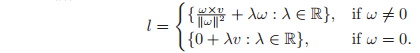
The axis l is a directed line through a point. For , the axis is a line in the direction going through the point . For , the axis is a line in the direction going through the origin. - Magnitude:
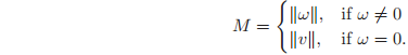
The magnitude of a screw is the net rotation if the motion contains a rotational component, or the net translation otherwise. If we choose (or when ), then a twist has magnitude .
We next show that given a screw, we can define a twist which realizes the screw motion and has the proper geometric attributes. It suffices to prove that we can define a twist with a given set of attributes, since any twist with those attributes will generate the correct screw motion.
Proposition 2.10. Screw motions correspond to twists
Given a screw with axis
, pitch
, and magnitude
, there exists a unit magnitude twist
such that the rigid motion associated with the screw is generated by the twist
.
There are several important special cases of screw motion of which we shall make frequent use. A zero pitch screw is a screw motion for which , corresponding to a pure rotation about an axis. Zero pitch screws are used to model the action of a revolute joint of a manipulator. The axis of the screw corresponds to the axis of rotation of the joint. An infinite pitch screw is a motion for which , as previously mentioned. This case corresponds to a pure translation and is the model for the action of a prismatic joint. The axis of the screw is defined to be a line through the origin which points in the direction of translation (a line through any other point could also be used). The magnitude of the screw gives the amount of the displacement. Finally, we define a unit twist to be a twist such that either , or and ; that is, a unit twist has magnitude . Unit twists are useful since they allow us to express rigid motions due to revolute and prismatic joints as exp( ), where corresponds to the amount of rotation or translation.
The formulas do not change for different choices of points on the axis of the screw. Thus, if is some other point on the axis of the screw, the formula in equation (2.40) would be unchanged.
Theorem 2.11 (Chasles). Every rigid body motion can be realized by a rotation about an axis combined with a translation parallel to that axis.
reference
A Mathematical Introduction to Robotic Manipulation Richard M. Murray, Zexiang Li, S. Shankar Sastry