Python----支持向量机SVM

1.1. SVM介绍

SVM（Support Vector Machines）——支持向量机。其含义是通过支持向量运算的分类器。其中“机”的意思是机器，可以理解为分类器。

1.2. 工作原理

在最大化支持向量到超平面距离前，我们首先要定义我们的超平面 $h (x)$

f(x) = w T x + b

核心思想：

首先通过两个分类的最近点，找到 $f (x)$
有了约束条件，就可以通过拉格朗日乘子法和KKT条件来求解，这时，问题变成了求拉格朗日乘子 $α_{i}$
对于异常点的情况，加入松弛变量 $ξ$
使用SMO来求拉格朗日乘子 $α_{i}$
惊喜! 不用求 $w$
非线性分类的问题：映射到高维度、使用核函数。

1.3. 实例

数据集：

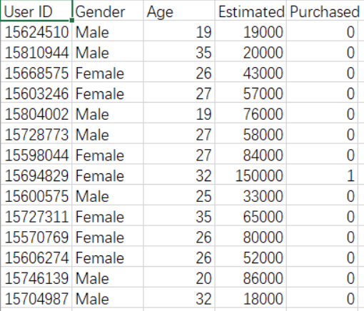
# Importing the libraries
import numpy as np
import matplotlib.pyplot as plt
import pandas as pd

# Importing the dataset
dataset = pd.read_csv('Social_Network_Ads.csv')
X = dataset.iloc[:, [2,3]].values
y = dataset.iloc[:, 4].values

# Splitting the dataset into the Training set and Test set
from sklearn.model_selection import train_test_split
X_train, X_test, y_train, y_test = train_test_split(X, y, test_size = 0.25, random_state = 0)

# Feature Scaling
from sklearn.preprocessing import StandardScaler
sc_X = StandardScaler()
X_train = sc_X.fit_transform(X_train)
X_test = sc_X.transform(X_test)

# Fitting Logistic Regression to the Training set
#训练集拟合SVM的分类器
#从模型的标准库中导入SVM的类
from sklearn.svm import SVC
classifier = SVC(kernel = 'linear', random_state = 0)
classifier.fit(X_train, y_train)

# Predicting the Test set results
#运用拟合好的分类器预测测试集的结果情况
#创建变量（包含预测出的结果）
y_pred = classifier.predict(X_test)

# Making the Confusion Matrix
#通过测试的结果评估分类器的性能
#用混淆矩阵，评估性能
#65,24对应着正确的预测个数；8,3对应错误预测个数；拟合好的分类器正确率：（65+24）/100
from sklearn.metrics import confusion_matrix
cm = confusion_matrix(y_test, y_pred)

# Visualising the Training set results
#在图像看分类结果
from matplotlib.colors import ListedColormap
#创建变量
X_set, y_set = X_train, y_train
#x1,x2对应图中的像素；最小值-1，最大值+1，-1和+1是为了让图的边缘留白，像素之间的距离0.01；第一行年龄，第二行年收入
X1, X2 = np.meshgrid(np.arange(start = X_set[:, 0].min() - 1, stop = X_set[:, 0].max() + 1, step = 0.01),
                     np.arange(start = X_set[:, 1].min() - 1, stop = X_set[:, 1].max() + 1, step = 0.01))
#将不同像素点涂色，用拟合好的分类器预测每个点所属的分类并且根据分类值涂色
plt.contourf(X1, X2, classifier.predict(np.array([X1.ravel(), X2.ravel()]).T).reshape(X1.shape),
             alpha = 0.75, cmap = ListedColormap(('red', 'green')))
#标注最大值及最小值
plt.xlim(X1.min(), X1.max())
plt.ylim(X2.min(), X2.max())
#为了滑出实际观测的点（黄、蓝）
for i, j in enumerate(np.unique(y_set)):
    plt.scatter(X_set[y_set == j, 0], X_set[y_set == j, 1],
                c = ListedColormap(('orange', 'blue'))(i), label = j)
plt.title('SVM (Training set)')
plt.xlabel('Age')
plt.ylabel('Estimated Salary')
#显示不同的点对应的值
plt.legend()
#生成图像
plt.show()

# Visualising the Test set results
from matplotlib.colors import ListedColormap
X_set, y_set = X_test, y_test
X1, X2 = np.meshgrid(np.arange(start = X_set[:, 0].min() - 1, stop = X_set[:, 0].max() + 1, step = 0.01),
                     np.arange(start = X_set[:, 1].min() - 1, stop = X_set[:, 1].max() + 1, step = 0.01))
plt.contourf(X1, X2, classifier.predict(np.array([X1.ravel(), X2.ravel()]).T).reshape(X1.shape),
             alpha = 0.75, cmap = ListedColormap(('red', 'green')))
plt.xlim(X1.min(), X1.max())
plt.ylim(X2.min(), X2.max())
for i, j in enumerate(np.unique(y_set)):
    plt.scatter(X_set[y_set == j, 0], X_set[y_set == j, 1],
                c = ListedColormap(('orange', 'blue'))(i), label = j)
plt.title('SVM (Test set)')
plt.xlabel('Age')
plt.ylabel('Estimated Salary')
plt.legend()
plt.show()

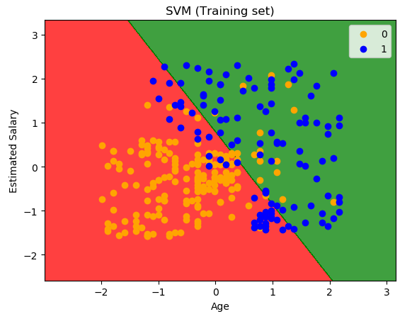
训练集图像显示结果：

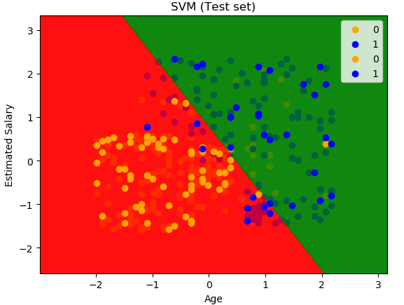
测试集图像显示结果

Python----支持向量机SVM

1.1. SVM介绍

1.2. 工作原理

1.3. 实例

猜你喜欢