1、LeNet-5模型简介
LeNet-5 模型是 Yann LeCun 教授于 1998 年在论文 Gradient-based learning applied to document
recognitionr [1] 中提出的,它是第一个成功应用于数字识别问题的卷积神经网络。在 MNIST 数据集
上, LeNet-5 模型可以达到大约 99.2%的正确率。
2、LeNet-5模型结构
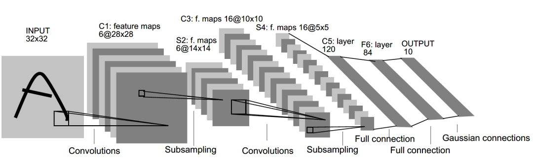
LeNet-5 模型总共有 7 层 ,下图展示了 LeNet-5 模型的架构 。
下面总结 LeNet-5 模型每一层的结构。
第一层: 卷积层
输入: 原始的图像像素矩阵(长、宽、色彩), 大小为 32*32*1。
卷积层参数: 过滤器尺寸为 5*5,深度为 6,不使用全 0 填充,步长为1。
输出:大小为 28*28*6。
分析:因为没有使用全 0 填充,所以这一层输出尺寸为 32-5+1=28, 深度为 6;
该卷积层共有 5*5*1*6+6=156 个参数,其中 6个为偏置项参数;
因为下一层的节点矩阵有 28*28*6=4704 个节点,每个节点和 5*5=25 个当前层节点相连,
所以本层卷积层共有 4704*(25+1)=122304 个连接。
第二层: 池化层
输入: 大小为 28*28*6。
池化层参数: 过滤器尺寸为 2*2,长和宽的步长均为2。
输出: 大小为 14*14*6
第三层: 卷积层
输入: 大小为 14*14*6。
卷积层参数: 过滤器尺寸为 5*5,深度为 16,不使用全 0 填充,步长为1。
输出:大小为 10*10*16。
分析:因为没有使用全 0 填充,所以这一层输出尺寸为 14-5+1=10, 深度为 16;
该卷积层共有 5*5*6*16+16=2416 个参数,其中 16个为偏置项参数;
因为下一层的节点矩阵有 10*10*16=1600 个节点,每个节点和 5*5=25 个当前层节点相连,
所以本层卷积层共有 1600*(25+1)=41600 个连接。
第四层: 池化层
输入: 大小为 10*10*16。
池化层参数: 过滤器尺寸为 2*2,长和宽的步长均为2。
输出: 大小为 5*5*16。
第五层: 全连接层
输入节点个数: 5*5*16=400。
参数个数: 5*5*16*120+120=48120 。
输出节点个数: 120。
第六层: 全连接层
输入节点个数: 120。
参数个数: 120*84+84=10164 。
输出节点个数: 84。
第七层: 全连接层
输入节点个数: 84。
参数个数: 84*10+10=850 。
输出节点个数: 10。
3、LeNet-5模型TensorFlow实现MNIST数字识别
开发环境: Python - 3.0、TensorFlow - 1.4.0、无GPU
训练主文件:LeNet5_train.py


# -*- coding: utf-8 -*-
"""
Created on 2017
《TensorFlow 实战Google深度学习框架 第2版 ,郑泽宇、梁博文等》
@author: 郑泽宇、梁博文等
"""
#见书 p151
#6.4.1 经典卷积神经网络模型——LeNet-5模型

import tensorflow as tf
from tensorflow.examples.tutorials.mnist import input_data
import LeNet5_infernece
import os
import numpy as np

BATCH_SIZE = 100     #每次选取batch_size个样本进行训练
TRAINING_STEPS = 6000   #训练次数
LEARNING_RATE_BASE = 0.01   #基础的学习率
global_step = tf.Variable(0, trainable=False)  #全局步长
LEARNING_RATE_DECAY = 0.99   #学习率的衰减率
REGULARIZATION_RATE = 0.0001   #正则化项系数
MOVING_AVERAGE_DECAY = 0.99  #滑动平均衰减率

def train(mnist):
    x = tf.placeholder(tf.float32, [
            BATCH_SIZE,
            LeNet5_infernece.IMAGE_SIZE,
            LeNet5_infernece.IMAGE_SIZE,
            LeNet5_infernece.NUM_CHANNELS],
        name='x-input')
    y_ = tf.placeholder(tf.float32, [None, LeNet5_infernece.OUTPUT_NODE], name='y-input')
    regularizer = tf.contrib.layers.l2_regularizer(REGULARIZATION_RATE)
    y = LeNet5_infernece.inference(x,False,regularizer)
    variable_averages = tf.train.ExponentialMovingAverage(MOVING_AVERAGE_DECAY, global_step)
    variables_averages_op = variable_averages.apply(tf.trainable_variables())

    cross_entropy = tf.nn.sparse_softmax_cross_entropy_with_logits(logits=y, labels=tf.argmax(y_, 1))
    cross_entropy_mean = tf.reduce_mean(cross_entropy)

    loss = cross_entropy_mean + tf.add_n(tf.get_collection('losses'))

    learning_rate = tf.train.exponential_decay(
        LEARNING_RATE_BASE,
        global_step,
        mnist.train.num_examples / BATCH_SIZE, LEARNING_RATE_DECAY,
        staircase=True)

    train_step = tf.train.GradientDescentOptimizer(learning_rate).minimize(loss, global_step=global_step)

    train_op = tf.group(train_step, variables_averages_op)
    saver = tf.train.Saver()

    with tf.Session() as sess:
        tf.global_variables_initializer().run()

        for i in range(TRAINING_STEPS):
            xs, ys = mnist.train.next_batch(BATCH_SIZE)
            reshaped_xs = np.reshape(xs, (
                BATCH_SIZE,
                LeNet5_infernece.IMAGE_SIZE,
                LeNet5_infernece.IMAGE_SIZE,
                LeNet5_infernece.NUM_CHANNELS))

            _, loss_value, step = sess.run([train_op, loss, global_step], feed_dict={x: reshaped_xs, y_: ys})
            if i % 1000 == 0:
                print("After %d training step(s), loss on training batch is %g." % (step, loss_value))

def main(argv=None):
    mnist = input_data.read_data_sets("MNIST_data", one_hot=True)
    train(mnist)

if __name__ == '__main__':
    main()
模型子文件:LeNet5_infernece.py
# -*- coding: utf-8 -*-
"""
Created on 2017
《TensorFlow 实战Google深度学习框架 第2版 ,郑泽宇》
@author: 郑泽宇、梁博文等
"""
#见书 p151
#6.4.1 经典卷积神经网络模型——LeNet-5模型

import tensorflow as tf

#1. 设定神经网络的参数
INPUT_NODE = 784
OUTPUT_NODE = 10

IMAGE_SIZE = 28
NUM_CHANNELS = 1

#第一层卷积层的尺寸和深度
CONV1_DEEP = 32  #第一层卷积层深度
CONV1_SIZE = 5  #第一层卷积层尺寸

#第二层卷积层的尺寸和深度
CONV2_DEEP = 64  #第二层卷积层深度
CONV2_SIZE = 5   #第二层卷积层尺寸

#第五层全连接层节点的个数
FC_SIZE = 512

#第六层全连接层节点的个数
NUM_LABELS = 10

#2. 定义前向传播的过程
#参数:输入(四维矩阵)、是否为训练/测试、正则化参数(参数变量管理)
def inference(input_tensor, train, regularizer):

    #声明第一层卷积层的变量并实现前向传播过程。
    #使用不同的命名空间来隔离不同层的变量。
    #输入: 28*28*1     输出: 28*28*32
    with tf.variable_scope('layer1-conv1'):
        #定义卷积过滤器。
        #定义卷积层参数:前两个为尺寸 5*5 、第三个为当前层节点矩阵的深度 1、第四个为卷积层的深度 32
        conv1_weights = tf.get_variable(
            "weight", [CONV1_SIZE, CONV1_SIZE, NUM_CHANNELS, CONV1_DEEP],
            initializer=tf.truncated_normal_initializer(stddev=0.1))
        #定义偏置项为 0,及下一层节点矩阵的深度 32(参数共享)
        conv1_biases = tf.get_variable("bias", [CONV1_DEEP], initializer=tf.constant_initializer(0.0))
        #tf.nn.conv2d 提供了一个方便的卷积层前向传播函数
        #参数1:当前层的节点矩阵,四维矩阵,第一维度对应一个输入batch,如第一张图片,第二张图片..
        #参数2:卷积层参数
        #参数3:不同维度上的步长(第一维、最后一维必须为1)
        #参数4:提供'SAME'和'VALLD'选择,'SAME'为添加全0填充,'VALLD'为不添加,填充的目的是矩阵尺寸在卷积层不变。
        conv1 = tf.nn.conv2d(input_tensor, conv1_weights, strides=[1, 1, 1, 1], padding='SAME')
        #tf.nn.bias_add提供给每个conv节点加上偏置项,再将计算结果通过ReLU激活函数完成去线性化
        relu1 = tf.nn.relu(tf.nn.bias_add(conv1, conv1_biases))

    #声明第二层池化层前向传播过程
    #使用不同的命名空间来隔离不同层的变量。
    #tf.nn.max_pool 提供了一个方便的最大池化层的前向传播过程。
    #tf.nn.avg_pool 提供了一个方便的平均池化层的前向传播过程,两者参数一致。
    #参数1:四维矩阵,第一维度对应一个输入batch,如第一张图片,第二张图片..
    #参数2:ksize为过滤器参数,常为[1, 2, 2, 1]、[1, 3, 3, 1]
    #参数3:不同维度上的步长(第一维、最后一维必须为1)
    #参数4:提供'SAME'和'VALLD'选择,'SAME'为添加全0填充,'VALLD'为不添加
    #输入: 28*28*32     输出: 14*14*32
    with tf.name_scope("layer2-pool1"):
        pool1 = tf.nn.max_pool(relu1, ksize = [1,2,2,1],strides=[1,2,2,1],padding="SAME")

    #声明第三层卷积层的变量并实现前向传播过程。
    #使用不同的命名空间来隔离不同层的变量。
    #输入: 14*14*32     输出: 14*14*64
    with tf.variable_scope("layer3-conv2"):
        conv2_weights = tf.get_variable(
            "weight", [CONV2_SIZE, CONV2_SIZE, CONV1_DEEP, CONV2_DEEP],
            initializer=tf.truncated_normal_initializer(stddev=0.1))
        conv2_biases = tf.get_variable("bias", [CONV2_DEEP], initializer=tf.constant_initializer(0.0))
        conv2 = tf.nn.conv2d(pool1, conv2_weights, strides=[1, 1, 1, 1], padding='SAME')
        relu2 = tf.nn.relu(tf.nn.bias_add(conv2, conv2_biases))

    #声明第四层池化层前向传播过程
    #输入: 14*14*64     输出: 7*7*64(不包括数据处理)
    with tf.name_scope("layer4-pool2"):
        pool2 = tf.nn.max_pool(relu2, ksize=[1, 2, 2, 1], strides=[1, 2, 2, 1], padding='SAME')
        pool_shape = pool2.get_shape().as_list()
        nodes = pool_shape[1] * pool_shape[2] * pool_shape[3]
        reshaped = tf.reshape(pool2, [pool_shape[0], nodes])

    #声明第五层全连接层的变量并实现前向传播过程
    #输入:向量长度为3136   输出:向量长度为512
    with tf.variable_scope('layer5-fc1'):
        fc1_weights = tf.get_variable("weight", [nodes, FC_SIZE],
                                      initializer=tf.truncated_normal_initializer(stddev=0.1))
        if regularizer != None: tf.add_to_collection('losses', regularizer(fc1_weights))
        fc1_biases = tf.get_variable("bias", [FC_SIZE], initializer=tf.constant_initializer(0.1))
        fc1 = tf.nn.relu(tf.matmul(reshaped, fc1_weights) + fc1_biases)
        if train: fc1 = tf.nn.dropout(fc1, 0.5)

    #声明第六层全连接层的变量并实现前向传播过程
    #输入:向量长度为512   输出:向量长度为10
    with tf.variable_scope('layer6-fc2'):
        fc2_weights = tf.get_variable("weight", [FC_SIZE, NUM_LABELS],
                                      initializer=tf.truncated_normal_initializer(stddev=0.1))
        if regularizer != None: tf.add_to_collection('losses', regularizer(fc2_weights))
        fc2_biases = tf.get_variable("bias", [NUM_LABELS], initializer=tf.constant_initializer(0.1))
        logit = tf.matmul(fc1, fc2_weights) + fc2_biases

    return logit
实验结果:
After 1 training step(s), loss on training batch is 5.95725.
After 1001 training step(s), loss on training batch is 0.664706.
After 2001 training step(s), loss on training batch is 0.670048.
After 3001 training step(s), loss on training batch is 0.638539.
After 4001 training step(s), loss on training batch is 0.743027.
After 5001 training step(s), loss on training batch is 0.638279.
MNIST数据集下载:
Yann LeCun's MNIST page 提供了 MNIST 训练集与测试集数据的下载。
下载后,解压在一个文件夹即可。
参考文献
[1] Lecun Y , Bottou L , Bengio Y , et al. Gradient-based learning applied to document recognition[J]. Proceedings of the IEEE, 1998, 86(11):2278-2324.
[2] 郑泽宇、梁博文等. TensorFlow 实战Google深度学习框架 第2版 [M] , 北京:电子工业出版社,2018.