卷积神经网络的常见网络结构
常见的架构图如下:
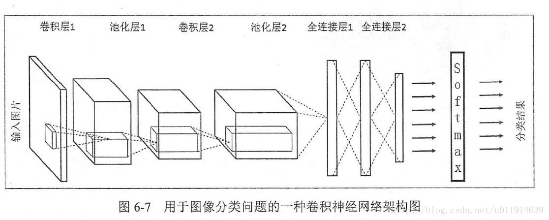
LeNet-5模型结构图如下图:

LeNet-5模型总共有7层。
第一层:卷积层
第一层卷积层的输入为原始的图像,原始图像的尺寸为32×32×1。卷积层的过滤器尺寸为5×5,深度为6,不使用全0补充,步长为1。由于没有使用全0补充,所以这一层的输出的尺寸为32-5+1=28,深度为6。这一个卷积层总共有5×5×1×6+6=156个参数,其中6为偏置项参数个数,卷积层的参数个数只和过滤器的尺寸,深度以及当前层节点矩阵的深度有关。因为下一层节点矩阵有28×28×6=4704个节点,每个节点和5×5=25个当前层节点相连,所以本层卷积层总共有4704×(25+1)=122304个连接。
第二层:池化层
这一层的输入为第一层的输出,是一个28×28×6的节点矩阵。本层采用的过滤器大小为2×2,步长为2,所以本层的输出矩阵大小为14×14×6。
第三层:卷积层
本层的输入矩阵大小为14×14×6,采用的过滤器大小为5×5,深度为16,不使用全0补充,步长为1。这一层的输出的尺寸为14-5+1=10,深度为16,即输出矩阵大小为10×10×16。本层参数有5×5×6×16+16=2416个,连接有10×10×16×(5×5+1)=41600个。
第四层:池化层
本层的输入矩阵大小为10×10×16,采用的过滤器大小为2×2,步长为2,本层的输出矩阵大小为5×5×16。
第五层:全连接层
本层的输入矩阵大小为5×5×16,在LeNet-5模型的论文中将这一层称为卷积层,但是因为过滤器的大小就是5×5,所以和全连接层没有区别,这里直接看成全连接层。本层输入为5×5×16矩阵,将其拉直为一个长度为5×5×16的向量,即将一个三维矩阵拉直到一维空间以向量的形式表示,这样才可以进入全连接层进行训练。本层的输出节点个数为120,所以总共有5×5×16×120+120=48120个参数。
第六层:全连接层
本层的输入节点个数为120个,输出节点个数为84个,总共有120×84+84=10164个参数。
第七层:全连接层
本层的输入节点个数为84个,输出节点个数为10个,总共有84×10+10=850个参数。
接下来以TensorFlow代码展示一个基于LeNet-5模型的mnist数字识别代码。
mnist数据集和完整代码下载链接为:https://download.csdn.net/download/casgj16/10698394 。
(1)mnist_inference.py 构建CNN网络
import  tensorflow as tf

INPUT_NODE=784
OUTPUT_NODE=10

NUM_CHANNELS=1

IMAGE_SIZE=28

CONV1_DEEP=6
CONV1_SIZE=5

CONV2_DEEP=16
CONV2_SIZE=5

FC_SIZE=120
FC2_SIZE=84

NUM_LABELS=10

#搭建CNN
def inference(input_tensor,train,regularizer):
    #第一层卷积层
    # 第一层:卷积层,过滤器的尺寸为5×5,深度为6,不使用全0补充,步长为1。
    # 尺寸变化:32×32×1->28×28×6
    with tf.variable_scope('layer1-conv1'):
        conv1_weights=tf.get_variable(
            "weight",[CONV1_SIZE,CONV1_SIZE ,NUM_CHANNELS,CONV1_DEEP],
            initializer=tf.truncated_normal_initializer(stddev=0.1)
        )
        conv1_biases=tf.get_variable(
            "biases",[CONV1_DEEP],initializer=tf.constant_initializer(0.0)
        )

        conv1=tf.nn.conv2d(
            input_tensor,conv1_weights,strides=[1,1,1,1],padding='VALID'
        )
        relu1=tf.nn.relu(tf.nn.bias_add(conv1,conv1_biases))

    # 第2层卷积层
    # 第二层:池化层,过滤器的尺寸为2×2,使用全0补充,步长为2。
    # 尺寸变化:28×28×6->14×14×6
    with tf.name_scope('layer2-pool1'):
        pool1=tf.nn.max_pool(
            relu1,ksize=[1,2,2,1],strides=[1,2,2,1],padding='SAME'
        )

    # 第三层:卷积层,过滤器的尺寸为5×5,深度为16,不使用全0补充,步长为1。
    # 尺寸变化:14×14×6->10×10×16
    with tf.variable_scope('layer3-conv2'):
        conv2_weights = tf.get_variable(
            "weight", [CONV2_SIZE, CONV2_SIZE, CONV1_DEEP, CONV2_DEEP],
            initializer=tf.truncated_normal_initializer(stddev=0.1)
        )
        conv2_biases = tf.get_variable(
            "biases", [CONV2_DEEP], initializer=tf.constant_initializer(0.0)
        )
        conv2 = tf.nn.conv2d(
            pool1, conv2_weights, strides=[1, 1, 1, 1], padding='VALID'
        )
        relu2 = tf.nn.relu(tf.nn.bias_add(conv2, conv2_biases))


    # 第四层:池化层,过滤器的尺寸为2×2,使用全0补充,步长为2。
    # 尺寸变化:10×10×6->5×5×16
    with tf.name_scope('layer4-pool2'):
        pool2 = tf.nn.max_pool(
            relu2, ksize=[1, 2, 2, 1], strides=[1, 2, 2, 1], padding='SAME'
        )

    # 将第四层池化层的输出转化为第五层全连接层的输入格式。
    # 第四层的输出为5×5×16的矩阵,然而第五层全连接层需要的输入格式
    # 为向量,所以我们需要把代表每张图片的尺寸为5×5×16的矩阵拉直成一个长度为5×5×16的向量。
    # 举例说,每次训练64张图片,
    # 那么第四层池化层的输出的size为(64,5,5,16),拉直为向量,
    # nodes=5×5×16=400,尺寸size变为(64,400)

    pool_shape=pool2.get_shape().as_list()
    nodes=pool_shape[1]*pool_shape[2]*pool_shape[3]
    reshaped = tf.reshape(pool2,[-1,nodes])


    # 第五层:全连接层,nodes=5×5×16=400,400->120的全连接
    # 尺寸变化:比如一组训练样本为64,那么尺寸变化为64×400->64×120
    # 训练时,引入dropout,dropout在训练时会随机将部分节点的输出改为0,
    # dropout可以避免过拟合问题。
    # 这和模型越简单越不容易过拟合思想一致,和正则化限制权重的大小,
    #   使得模型不能任意拟合训练数据中的随机噪声,以此达到避免过拟合思想一致。
    # 本文最后训练时没有采用dropout,
    # dropout项传入参数设置成了False,因为训练和测试写在了一起没有分离,不过大家可以尝试。
    with tf.variable_scope('layer5-fc1'):
        fc1_weights=tf.get_variable(
            "weight",[nodes,FC_SIZE],
            initializer=tf.truncated_normal_initializer(stddev=0.1)
        )
        if regularizer!=None:
            tf.add_to_collection('losses',regularizer(fc1_weights))
        fc1_biases=tf.get_variable(
            "biases",[FC_SIZE],initializer=tf.constant_initializer(0.1)
        )

        fc1=tf.nn.relu(tf.matmul(reshaped,fc1_weights)+fc1_biases)
        if train:
            fc1=tf.nn.dropout(fc1,0.5)


    # 第六层:全连接层,120->84的全连接
    # 尺寸变化:比如一组训练样本为64,那么尺寸变化为64×120->64×84
    with tf.variable_scope('layer6-fc2'):
        fc2_weights=tf.get_variable(
            "weight",[FC_SIZE,FC2_SIZE],
            initializer=tf.truncated_normal_initializer(stddev=0.1)
        )
        if regularizer!=None:
            tf.add_to_collection('losses',regularizer(fc2_weights))
        fc2_biases = tf.get_variable(
            'biases',
            [FC2_SIZE],
            initializer=tf.truncated_normal_initializer(stddev=0.1)
        )
        fc2 = tf.nn.relu(tf.matmul(fc1, fc2_weights) + fc2_biases)
        if train:
            fc2 = tf.nn.dropout(fc2, 0.5)


    #第七层:全连接层(近似表示),84->10的全连接
    #尺寸变化:比如一组训练样本为64,那么尺寸变化为64×84->64×10。
    # 最后,64×10的矩阵经过softmax之后就得出了64张图片分类于每种数字的概率,
    #即得到最后的分类结果。
    with tf.variable_scope('layer7-fc3'):
        fc3_weights = tf.get_variable(
            'weight',[FC2_SIZE,NUM_LABELS],
            initializer=tf.truncated_normal_initializer(stddev=0.1)
        )
        if regularizer != None:
            tf.add_to_collection('losses',regularizer(fc3_weights))
        fc3_biases = tf.get_variable('biases',
                                     [NUM_LABELS],
                                     initializer=tf.truncated_normal_initializer(stddev=0.1)
                                     )
        logit = tf.matmul(fc2,fc3_weights) + fc3_biases
    return logit
(2)mnist_train.py训练和测试
from skimage import io,transform
import os
import glob
import numpy as np
import tensorflow as tf
import mnist_inference
#将所有的图片重新设置尺寸为32*32
w = 32
h = 32

#mnist数据集中训练数据和测试数据保存地址
train_path = "C:/Users/mnist/train/"
test_path = "C:/Users/mnist/test/"

#读取图片及其标签函数
def read_image(path):
    label_dir = [path+x for x in os.listdir(path) if os.path.isdir(path+x)]
    images = []
    labels = []
    for index,folder in enumerate(label_dir):
        for img in glob.glob(folder+'/*.png'):
            print("reading the image:%s"%img)
            image = io.imread(img)
            image = transform.resize(image,(w,h,mnist_inference.NUM_CHANNELS))
            images.append(image)
            labels.append(index)
    return np.asarray(images,dtype=np.float32),np.asarray(labels,dtype=np.int32)


#读取训练数据及测试数据
train_data,train_label = read_image(train_path)
test_data,test_label = read_image(test_path)

#打乱训练数据及测试数据
train_image_num = len(train_data)
train_image_index = np.arange(train_image_num)
np.random.shuffle(train_image_index)
train_data = train_data[train_image_index]
train_label = train_label[train_image_index]

test_image_num = len(test_data)
test_image_index = np.arange(test_image_num)
np.random.shuffle(test_image_index)  #numpy.random.shuffle打乱顺序函数

test_data = test_data[test_image_index]
test_label = test_label[test_image_index]

#输入
x = tf.placeholder(tf.float32,[None,w,h,mnist_inference.NUM_CHANNELS],name='x')
y_ = tf.placeholder(tf.int32,[None],name='y_')


#-------构建CNN---------------------
#正则化,交叉熵,平均交叉熵,损失函数,最小化损失函数,预测和实际equal比较,tf.equal函数会得到True或False,
#正则化
regularizer = tf.contrib.layers.l2_regularizer(0.001)
#前向网络结果
y = mnist_inference.inference(x,False,regularizer)
#损失函数
cross_entropy = tf.nn.sparse_softmax_cross_entropy_with_logits(logits=y,labels=y_)
cross_entropy_mean = tf.reduce_mean(cross_entropy)
loss = cross_entropy_mean + tf.add_n(tf.get_collection('losses'))
#最小化损失函数
train_op = tf.train.AdamOptimizer(0.001).minimize(loss)
#accuracy首先将tf.equal比较得到的布尔值转为float型,即True转为1.,False转为0,
# 最后求平均值,即一组样本的正确率。
#比如:一组5个样本,tf.equal比较为[True False True False False],
# 转化为float型为[1.  0   1.  0  0],准确率为2./5=40%。
correct_prediction = tf.equal(tf.cast(tf.argmax(y,1),tf.int32),y_)
accuracy = tf.reduce_mean(tf.cast(correct_prediction,tf.float32))


#每次获取batch_size个样本进行训练或测试
def get_batch(data,label,batch_size):
    for start_index in range(0,len(data)-batch_size+1,batch_size):
        slice_index = slice(start_index,start_index+batch_size)
        yield data[slice_index],label[slice_index]


#创建Session会话
with tf.Session() as sess:
    #初始化所有变量(权值,偏置等)
    sess.run(tf.global_variables_initializer())

    #将所有样本训练10次,每次训练中以64个为一组训练完所有样本。
    #train_num可以设置大一些。
    train_num = 10
    batch_size = 64

    for i in range(train_num):

        train_loss,train_acc,batch_num = 0, 0, 0

        for train_data_batch, train_label_batch in get_batch(train_data, train_label, batch_size):
            _, err, acc = sess.run([train_op, loss, accuracy], feed_dict={x: train_data_batch, y_: train_label_batch})
            train_loss += err;
            train_acc += acc;
            batch_num += 1

        print("train loss:", train_loss / batch_num)
        print("train acc:", train_acc / batch_num)

        test_loss,test_acc,batch_num = 0, 0, 0
        for test_data_batch,test_label_batch in get_batch(test_data,test_label,batch_size):
            err2,acc2 = sess.run(
                [loss,accuracy],
                feed_dict={x:test_data_batch,y_:test_label_batch}
            )
            test_loss += err;
            test_acc += acc;
            batch_num += 1
        print("test loss:", test_loss / batch_num)
        print("test acc:", test_acc / batch_num)
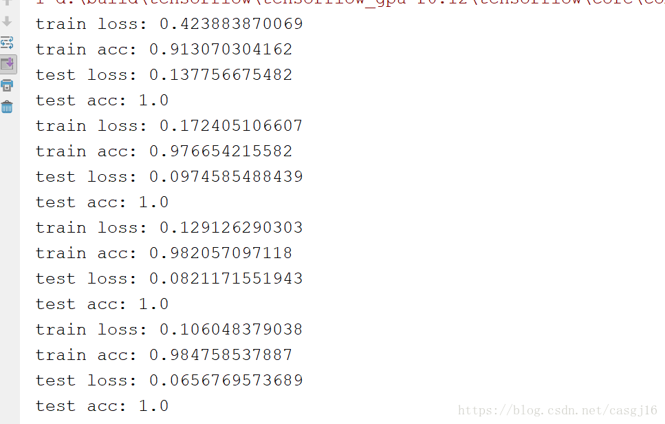
(3)实验结果