不写点东西学了都忘了
这是一个简单的拟合线性回归的例子,若有错误和疑问欢迎指出!
深度学习的步骤大概分为以下四个:
- 准备数据
- 搭建模型
- 迭代训练
- 使用模型
分享连接
numpy模块的中文学习链接
matplotlib官网学习链接(可借助翻译软件学习)
Anaconda3.5.1 tensorflow-gpu==1.13.1 CUDA10 Cudnn7.5 安装教程
numpy、matplotlib模块pip安装教程
一,准备数据
这个步骤实现两个功能:
- 引入头文件
- 生成带噪音的数据点
import tensorflow as tf #导入tensorflow模块
import numpy as np #导入numpy模块
import matplotlib.pyplot as plt #导入matplotlib模块中的pyplot模块并重命名为plt
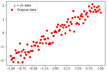
train_X = np.linspace(-1,1,100) #在-1 ~ 1中生成100个数据点train_X
train_Y = 2 * train_X + np.random.randn(*train_X.shape) * 0.3 #y = 2x,但是加入了本身乘上0.3的早生
#提示:下面的ro是plot函数中的format_string参数,r-红色,o-实心圈标记
plt.plot(train_X,train_Y,'ro',label = 'Original data')#显示模拟的数据点
plt.legend(title = 'y = 2x data') #数据点适应大小,图例标题:y = 2x data
plt.show()
代码效果:
二,搭建模型
1,正向搭建模型
这个步骤是为了实现模型的正向传输,类似于,输入x,然后得出y,相当于模拟使用
#create the model
#------------------------------
#set the placeholders
X = tf.placeholder('float')
Y = tf.placeholder('float')
#set model's parameter
W = tf.Variable(tf.random_normal([1]),name = 'weight') #weight:权重
b = tf.Variable(tf.zeros([1]),name = 'bias')  #bias:偏向
#forward structure
z = tf.multiply(X,W) + b
#reverse optimization
cost = tf.reduce_mean(tf.square(Y - z))
learning_rate = 0.01
optimizer = tf.train.GradientDescentOptimizer(learning_rate).minimize(cost)
#----------------------------------------------------------------------------
2,反向搭建播型
这个步骤是为了通过由正向模型计算出的值与标签(我们希望生成的值)进行参数(W:权重与b:偏
差)调整,然后使模型的输出越来越符合我们期望生成的值
#reverse optimization
cost = tf.reduce_mean(tf.square(Y - z))
learning_rate = 0.01
optimizer = tf.train.GradientDescentOptimizer(learning_rate).minimize(cost)
三,迭代训练
1,训练模型
tensorflow中的任务通过session进行,全局初始化变量,设定迭代次数,启动session进行训练
#lterative training model
#---------------------------
#Initialize all variables
init = tf.global_variables_initializer()
#set the parameter
training_epochs = 20
display_step = 2
#start session
with tf.Session() as sess:
sess.run(init)
plotdata = {"batchsize":[],"loss":[]} #Storage batch value and loss value
#input data to the model
for epoch in range(training_epochs):
for (x,y) in zip(train_X,train_Y):
sess.run(optimizer,feed_dict = {X:x,Y:y})
if epoch % display_step == 0:
loss = sess.run(cost,feed_dict = {X:train_X,Y:train_Y})
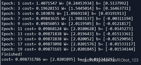
print ("Epoch:", epoch+1, "cost=", loss,"W=", sess.run(W), "b=", sess.run(b))
if not (loss =="NA"):
plotdata["batchsize"].append(epoch)
plotdata["loss"].append(loss)
print("Finished!")
print ("cost=", sess.run(cost, feed_dict={X: train_X, Y: train_Y}), "w=", sess.run(W), "b=", sess.run(b))
运行效果:
2,模型可视化
#show in picture
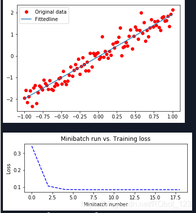
plt.plot(train_X,train_Y,'ro',label='Original data')
plt.plot(train_X,sess.run(W) * train_X + sess.run(b),label = 'Fittedline')
plt.legend()
plt.show()
plotdata["avgloss"] = moving_average(plotdata["loss"])
plt.figure(1)
plt.subplot(211)
plt.plot(plotdata['batchsize'],plotdata['avgloss'],'b--')
plt.xlabel('Minibatch number')
plt.ylabel('Loss')
plt.title('Minibatch run vs. Training loss')
plt.show()
运行效果:
四,使用模型
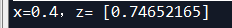
#use the model
    print ("x=0.4,z=", sess.run(z, feed_dict={X: 0.4}))
运行效果:
五,完整代码
# -*- coding: utf-8 -*-
"""
Created on Sun Dec  8 16:41:37 2019

@author: HPN
CSDN博客:https://blog.csdn.net/RObot_123
"""

import tensorflow as tf      #导入tensorflow模块
import numpy as np           #导入numpy模块
import matplotlib.pyplot as plt #导入matplotlib模块中的pyplot模块并重命名为plt

plotdata = { "batchsize":[], "loss":[] }
def moving_average(a, w=10):
    if len(a) < w:
        return a[:]
    return [val if idx < w else sum(a[(idx-w):idx])/w for idx, val in enumerate(a)]


train_X = np.linspace(-1,1,100)    #在-1 ~ 1中生成100个数据点train_X
train_Y = 2 * train_X + np.random.randn(*train_X.shape) * 0.3 #y = 2x,但是加入了本身乘上0.3的早生

#提示:下面的ro是plot函数中的format_string参数,r-红色,o-实心圈标记
plt.plot(train_X,train_Y,'ro',label = 'Original data')#显示模拟的数据点
plt.legend(title = 'y = 2x data')   #数据点适应大小,图例标题:y = 2x data
plt.show()                          #显示图片

#create the model
#------------------------------
#set the placeholders
X = tf.placeholder('float')
Y = tf.placeholder('float')
#set model's parameter
W = tf.Variable(tf.random_normal([1]),name = 'weight') #weight:权重
b = tf.Variable(tf.zeros([1]),name = 'bias')  #bias:偏向
#forward structure
z = tf.multiply(X,W) + b
#reverse optimization
cost = tf.reduce_mean(tf.square(Y - z))
learning_rate = 0.01
optimizer = tf.train.GradientDescentOptimizer(learning_rate).minimize(cost)
#----------------------------------------------------------------------------

#lterative training model
#---------------------------
#Initialize all variables
init = tf.global_variables_initializer()
#set the parameter
training_epochs = 20
display_step = 2
#start session
with tf.Session() as sess:
    sess.run(init)
    plotdata = {"batchsize":[],"loss":[]} #Storage batch value and loss value
    #input data to the model
    for epoch in range(training_epochs):
        for (x,y) in zip(train_X,train_Y):
            sess.run(optimizer,feed_dict = {X:x,Y:y})
        if epoch % display_step == 0:
            loss = sess.run(cost,feed_dict = {X:train_X,Y:train_Y})
            print ("Epoch:", epoch+1, "cost=", loss,"W=", sess.run(W), "b=", sess.run(b))
            if not (loss =="NA"):
                plotdata["batchsize"].append(epoch)
                plotdata["loss"].append(loss)
    print("Finished!")
    print ("cost=", sess.run(cost, feed_dict={X: train_X, Y: train_Y}), "w=", sess.run(W), "b=", sess.run(b))

#show in picture
    plt.plot(train_X,train_Y,'ro',label='Original data')
    plt.plot(train_X,sess.run(W) * train_X + sess.run(b),label = 'Fittedline')
    plt.legend()
    plt.show()

    plotdata["avgloss"] = moving_average(plotdata["loss"])
    plt.figure(1)
    plt.subplot(211)
    plt.plot(plotdata['batchsize'],plotdata['avgloss'],'b--')
    plt.xlabel('Minibatch number')
    plt.ylabel('Loss')
    plt.title('Minibatch run vs. Training loss')
    plt.show()

#use the model
    print ("x=0.4,z=", sess.run(z, feed_dict={X: 0.4}))
总结:这个拟合模型用到了numpy、matplotlib模块,其中的细节需要翻看网上的资料,具体学习链接在文章开头
