Python计算机视觉编程第一章——基本的图像操作和处理

基本的图像操作和处理

（一）PIL：Python 图像处理类库

PIL（Python Imaging Library Python，图像处理类库）提供了通用的图像处理功能， 以及大量有用的基本图像操作，比如图像缩放、裁剪、旋转、颜色转换等。虽然PIL是python的第三方图像处理库，但是由于其强大的功能与众多的使用人数，几乎已经被认为是python官方图像处理库了。

下面介绍PIL Image类中常用的函数:

open(filename,mode)                                           #读取一张图像

convert(mode,matrix,dither,palette,colors)          #图像的颜色转换

编写代码：

from PIL import Image
from pylab import *
pil_im = Image.open('D:\\Python\\chapterone\\dog.jpg')
gray()
subplot(131)
title('(a)')
axis('off')
imshow(pil_im)
pil_i = Image.open('D:\\Python\\chapterone\\dog.jpg').convert('L')        #图像转换为灰度图像
subplot(132)
title('(b)')
axis('off')
imshow(pil_i)
im_rgb = pil_i.convert("RGB")       #灰度图像转换为RGB图像
subplot(133)
title('(c)')
axis('off')
imshow(im_rgb)
show()

代码运行效果如下：

分析：

convert方法可以改变图像的mode,一般是在’RGB’(真彩图)、‘L’(灰度图)、‘CMYK’(压缩图)之间转换。上面的代码就是首先将图像转化为灰度图，再从灰度图转化为真彩图。值得注意的是,从灰度图转换为真彩图，虽然理论上确实转换成功了，但是实际上是很难恢复成原来的真彩模式的。

1.1 转换图像格式

通过 save() 方法，PIL 可以将图像保存成多种格式的文件。

函数：

扫描二维码关注公众号，回复： 8878517 查看本文章

save(filename,format)

编写代码：

from PIL import Image
from pylab import *
im = Image.open('D:\\Python\\chapterone\\dog.jpg', "r")
dog = im.save('D:\\Python\\chapterone\\dog.png', 'png')
dog.show()

代码运行效果如下：

分析：

上面的代码将jpg图像重新保存成png格式。注意，保存文件的文件名很重要，除非指定格式，否则这个库将会以文件名的扩展名作为格式保存。

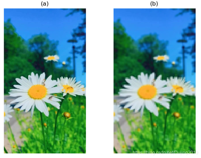
1.2 创建缩略图

Image 类的 thumbnail() 方法可以用来制作缩略图。它接受一个二元数组作为缩略图的尺寸，然后将示例缩小到指定尺寸。

函数：

thumbnail(size,resample)

thumbnail方法是原地操作，返回值是None。第一个参数是指定的缩略图的大小，第二个是采样的，有Image.BICUBIC，PIL.Image.LANCZOS，PIL.Image.BILINEAR，PIL.Image.NEAREST这四种采样方法。默认是Image.BICUBIC。

编写代码：

from PIL import Image
from pylab import *
im = Image.open('D:\\Python\\chapterone\\flower5.jpg', "r")
subplot(121)
title('(a)')
axis('off')
imshow(im)

im.save('D:\\Python\\chapterone\\flower5.png', 'png')
im.thumbnail((128, 128), resample=Image.BICUBIC)
subplot(122)
title('(b)')
axis('off')
imshow(im)
show()

代码运行效果如下：

编写代码：

from PIL import Image
from pylab import *
im = Image.open('D:\\Python\\chapterone\\flower5.jpg', "r")
im.save('D:\\Python\\chapterone\\flower5.png', 'png')
im.show()
im.thumbnail((128, 128), resample=Image.BICUBIC)
im.show()

代码运行效果如下：

分析：

从第一幅图可以看出，创建最长边为 128 像素的缩略图，图像在同样大小的情况下展示，会变得模糊，从第二幅图可以看出，正常情况下展示指定像素的缩略图，图像会变小。

1.3 复制和粘贴图像区域

使用 crop() 方法可以从一幅图像中裁剪指定区域：

函数：

crop(box)

编写代码：

from PIL import Image
from pylab import *
im = Image.open('D:\\Python\\chapterone\\flower5.jpg', "r")
subplot(121)
title('(a)')
axis('off')
imshow(im)

box = (100,500,400,700)
subplot(122)
title('(b)')
axis('off')
imshow(im.crop(box))
show()

代码运行效果如下：

分析：

上面的代码在im图像上裁剪了一个box矩形区域，然后显示出来。box是一个有四个数字的元组(upper_left_x,upper_left_y,lower_right_x,lower_right_y),分别表示裁剪矩形区域的左上角x,y坐标,右下角的x,y坐标,规定图像的最左上角的坐标为原点(0,0),宽度的方向为x轴，高度的方向为y轴，每一个像素代表一个坐标单位。crop()返回的仍然是一个Image对象。

paste() 方法则可以将一个 Image 示例粘贴到另一个 Image 示例上。

函数：

paste(region,box,mask)

编写代码：

from PIL import Image
from pylab import *
im = Image.open('D:\\Python\\chapterone\\flower5.jpg', "r")
subplot(131)
title('(a)')
axis('off')
imshow(im)

box = (100,500,400,700)
subplot(132)
title('(b)')
axis('off')
imshow(im.crop(box))

region = im.crop(box)
im.paste(region,(300,200),None)
subplot(133)
title('(c)')
axis('off')
imshow(im)
show()

代码运行效果如下：

分析:

上面的代码将region图像粘贴到左上角为(300,200)的位置（也就是雏菊图像的右上角）。region是要粘贴的Image对象,box是要粘贴的位置，可以是一个两个元素的元组，表示粘贴区域的左上角坐标,也可以是一个四个元素的元组，表示左上角和右下角的坐标。如果是四个元素元组的话,box的size必须要和region的size保持一致，否则将会被转换成和region一样的size。

1.4 调整尺寸和旋转

transpose() 方法可以将图片左右颠倒、上下颠倒、旋转 90°、旋转 180° 或旋转 270°

函数：

transpose(method)                #method表示选择什么样的翻转或者旋转方式

编写代码：

from PIL import Image
from pylab import *
im = Image.open('D:\\Python\\chapterone\\lovely2.jpg', "r")
subplot(331)
title('(a)')
axis('off')
imshow(im)

Image.FLIP_LEFT_RIGHT = im.transpose(Image.FLIP_LEFT_RIGHT)
subplot(332)
title('(b)')
axis('off')
imshow(Image.FLIP_LEFT_RIGHT)

Image.FLIP_TOP_BOTTOM = im.transpose(Image.FLIP_TOP_BOTTOM)
subplot(333)
title('(c)')
axis('off')
imshow(Image.FLIP_TOP_BOTTOM)

Image.ROTATE_45 = im.rotate(45)
subplot(334)
title('(d)')
axis('off')
imshow(Image.ROTATE_45)

Image.ROTATE_90 = im.transpose(Image.ROTATE_90)
subplot(335)
title('(e)')
axis('off')
imshow(Image.ROTATE_90)

Image.ROTATE_180 = im.transpose(Image.ROTATE_180)
subplot(336)
title('(f)')
axis('off')
imshow(Image.ROTATE_180)

Image.ROTATE_270 = im.transpose( Image.ROTATE_270)
subplot(337)
title('(g)')
axis('off')
imshow( Image.ROTATE_270)

Image.TRANSPOSE = im.transpose(Image.TRANSPOSE)
subplot(338)
title('(h)')
axis('off')
imshow(Image.TRANSPOSE)

Image.TRANSVERSE = im.transpose(Image.TRANSVERSE)
subplot(339)
title('(i)')
axis('off')
imshow(Image.TRANSVERSE)

show()

代码运行效果如下：

分析：
( b ) Image.FLIP_LEFT_RIGHT,表示将图像左右翻转
( c ) Image.FLIP_TOP_BOTTOM,表示将图像上下翻转
( d ) rotate(45)，表示将图像逆时针旋转45°
( e ) Image.ROTATE_90,表示将图像逆时针旋转90°
( f ) Image.ROTATE_180,表示将图像逆时针旋转180°
( g ) Image.ROTATE_270,表示将图像逆时针旋转270°
( h ) Image.TRANSPOSE,表示将图像进行转置(相当于顺时针旋转90°)
( i ) Image.TRANSVERSE,表示将图像进行转置,再水平翻转

要调整一幅图像的尺寸，可以调用 resize() 方法。该方法的参数是一个元组， 用来指定新图像的大小：

函数：

resize(size,resample,box)

编写代码：

from PIL import Image
from pylab import *
im = Image.open('D:\\Python\\chapterone\\lovely.jpg', "r")
im.show()
im_resize = im.resize((200,200))
im_resize.show()
im_resize_box = im.resize((100,100),box = (300,250,700,700))
im_resize_box.show()

代码运行效果如下：

分析：

resize方法可以将原始的图像转换大小,size是转换之后的大小,可以看出图像越来越小，resample是重新采样使用的方法，仍然有Image.BICUBIC，PIL.Image.LANCZOS，PIL.Image.BILINEAR，PIL.Image.NEAREST这四种采样方法，默认是PIL.Image.NEAREST,box是指定的要resize的图像区域（卡通人物的嘴巴部分），是一个用四个元组指定的区域(含义和上面所述box一致)。

（二）Matplotlib

处理数学运算、绘制图表，或者在图像上绘制点、直线和曲线时，Matplotlib 是个很好的类库，具有比 PIL 更强大的绘图功能。Matplotlib 可以绘制出高质量的 图表，就像本书中的许多插图一样。Matplotlib 中的 PyLab 接口包含很多方便用户 创建图像的函数。Matplotlib 是开源工具，可以从http://matplotlib.sourceforge.net/ 免费下载。

2.1 绘制图像、点和线

编写代码：

# coding:utf-8
import matplotlib.pyplot as plt
import matplotlib.ticker as ticker

x = ['2019-05-01', '2019-05-02', '2019-05-03', '2019-05-04', '2019-05-05'
     , '2019-05-06', '2019-05-07', '2019-05-08', '2019-05-09', '2019-05-10']
y = [1, 1, 2, 3, 4, 6, 7, 9, 11, 16]
z = [1, 2, 3, 4, 7, 9, 12, 13, 15, 20]
# 设置画布大小
plt.figure(figsize=(20, 4))

tick_spacing = 4
fig, ax = plt.subplots(1, 1)
ax.xaxis.set_major_locator(ticker.MaxNLocator(tick_spacing))

# 标题
plt.title("title")
# 横坐标描述
plt.xlabel('date')
# 纵坐标描述
plt.ylabel('num')

# 这里设置线宽、线型、线条颜色、点大小等参数
ax.plot(x, y, label='yy', linewidth=2, color='g', marker='o', markerfacecolor='red', markersize=4)
ax.plot(x, z, label='zz', linewidth=2, color='y', marker='o', markerfacecolor='black', markersize=4)
# 每个数据点加标签
for a, b in zip(x, z):
    plt.text(a, b, str(b)+'%', ha='center', va='bottom', fontsize=12)
# 只给最后一个点加标签
plt.text(x[-1], y[-1], y[-1], ha='center', va='bottom', fontsize=15)

# 旋转x轴标签
for label in ax.get_xticklabels():
     label.set_rotation(30)  # 旋转30度
     label.set_horizontalalignment('right')  # 向右旋转

# 图例显示及位置确定
plt.legend(loc='upper left')
plt.savefig('D:\\Python\\chapterone\\lovely2.jpg', bbox_inches='tight')
plt.show()

代码运行效果如下：

补充：

plot(x, y) # 默认为蓝色实线
plot(x, y, ‘r*’) # 红色星状标记
plot(x, y, ‘go-’) # 带有圆圈标记的绿线
plot(x, y, ‘ks:’) # 带有正方形标记的黑色点线

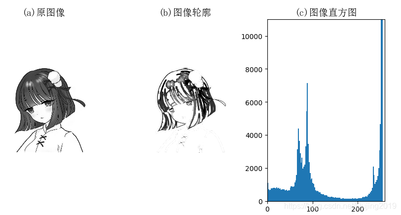
2.2 图像轮廓和直方图

在画图像轮廓前需要转换为灰度图像，因为轮廓需要获取每个坐标[x,y]位置的像素值。绘图都可以调用matplotlib.pyplot库来进行，其中的hist函数可以直接绘制直方图。

函数：

n, bins, patches = plt.hist(arr, bins, normed, facecolor, alpha)

hist的参数非常多，但常用的就这五个，只有第一个是必须的，后面四个可选。

arr: 需要计算直方图的一维数组
bins: 直方图的柱数，可选项，默认为10
normed: 是否将得到的直方图向量归一化。默认为0
facecolor: 直方图颜色
alpha: 透明度

返回值 ：

n: 直方图向量，是否归一化由参数设定
bins: 返回各个bin的区间范围
patches: 返回每个bin里面包含的数据，是一个list

灰度直方图：
编写代码：

# -*- coding: utf-8 -*-
from PIL import Image
from pylab import *

# 添加中文字体支持
from matplotlib.font_manager import FontProperties
font = FontProperties(fname=r"c:\windows\fonts\SimSun.ttc", size=14)
im = array(Image.open("D:\\Python\\chapterone\\girl2.jpg").convert('L'))  # 打开图像，并转成灰度图像

figure()

subplot(131)
axis('off')
imshow(im)
axis('equal')
axis('off')
title(u'(a)原图像', fontproperties=font)

# 使用颜色信息
subplot(132)
gray()
# 在原点的左上角显示轮廓图像
contour(im, origin='image')
axis('equal')
axis('off')
title(u'(b)图像轮廓', fontproperties=font)

subplot(133)
hist(im.flatten(), 128)
title(u'(c)图像直方图', fontproperties=font)
plt.xlim([0,260])
plt.ylim([0,11000])

show()

代码运行效果如下：

彩色图像直方图：
编写代码：

# -*- coding: utf-8 -*-
from PIL import Image
import numpy as np
import matplotlib.pyplot as plt
from pylab import *

from matplotlib.font_manager import FontProperties
font = FontProperties(fname=r"c:\windows\fonts\SimSun.ttc", size=14)
im=Image.open('D:\\Python\\chapterone\\dog1.jpg')
r,g,b=im.split()
figure()
subplot(121)
title(u'(a)原图像', fontproperties=font)
axis('off')
imshow(im)
axis('equal')
axis('off')

subplot(122)
title(u'(b)图像直方图', fontproperties=font)
ar=np.array(r).flatten()
plt.hist(ar, bins=256, normed=1,facecolor='yellowgreen',edgecolor='yellowgreen',hold=1)
ag=np.array(g).flatten()
plt.hist(ag, bins=256, normed=1, facecolor='pink',edgecolor='pink',hold=1)
ab=np.array(b).flatten()
plt.hist(ab, bins=256, normed=1, facecolor='deepskyblue',edgecolor='deepskyblue')
plt.show()
show()

代码运行效果如下：

分析：
彩色直方图实际上是和灰度直方图一样的，只是分别画出三通道的直方图，然后叠加在一起。不过从这可以看出，matplotlib的画图功能是非常强大的。

2.3 交互式标注

有时用户需要和某些应用交互，例如在一幅图像中标记一些点，或者标注一些训练数据。PyLab 库中的 ginput() 函数就可以实现交互式标注。

编写代码：

from PIL import Image
from pylab import *

im = array(Image.open('D:\\Python\\chapterone\\girl.jpg'))
imshow(im)
print 'Please click 3 points'
x = ginput(3)
print 'you clicked:', x
show()

出现问题：
在图像上标记点，x返回值仍为空。

解决方案：
具体：Settings | Tools | Python Scientific | Show Plots in Toolwindow，去掉对勾

代码运行效果如下：

在绘图窗口的图像区域点击三次。程序将这些点击的坐标 [x, y] 自动保存在 x 列表里。

（三）NumPy

NumPy（http://www.scipy.org/NumPy/）是非常有名的 Python 科学计算工具包，其中 包含了大量有用的思想，比如数组对象（用来表示向量、矩阵、图像等）以及线性 代数函数。NumPy 中的数组对象几乎贯穿用于本书的所有例子中 1 数组对象可以帮助 你实现数组中重要的操作，比如矩阵乘积、转置、解方程系统、向量乘积和归一化， 这为图像变形、对变化进行建模、图像分类、图像聚类等提供了基础。NumPy 可以从http://www.scipy.org/Download 免费下载。

3.1 图像数组表示

NumPy 中的数组对象是多维的，可以用来表示向量、矩阵和图像。一个数组对象很像一个列表（或者是列表的列表），但是数 组中所有的元素必须具有相同的数据类型。除非创建数组对象时指定数据类型，否则数据类型会按照数据的类型自动确定。

编写代码：

from PIL import Image
from pylab import *

im = array(Image.open('D:\\Python\\chapterone\\girl.jpg'))
print im.shape, im.dtype
im = array(Image.open('D:\\Python\\chapterone\\girl.jpg').convert('L'),'f')
print im.shape, im.dtype

代码运行效果如下：

分析：

每行的第一个元组表示图像数组的大小（行、列、颜色通道），紧接着的字符串表 示数组元素的数据类型。因为图像通常被编码成无符号八位整数（uint8），所以在第一种情况下，载入图像并将其转换到数组中，数组的数据类型为“uint8”。在第二种情况下，对图像进行灰度化处理，并且在创建数组时使用额外的参数“f”；该参数将数据类型转换为浮点型。

3.2 灰度变换

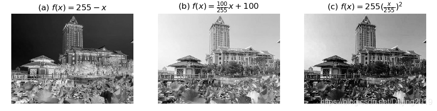
将图像读入 NumPy 数组对象后，我们可以对它们执行任意数学操作。一个简单的例子就是图像的灰度变换。

 # -*- coding: utf-8 灰度变换-*-
from PIL import Image
from numpy import *
from pylab import *

im = array(Image.open("D:\\Python\\chapterone\\jimei2.png").convert('L'))
print int(im.min()), int(im.max())

im2 = 255 - im  # 对图像进行反相处理
print int(im2.min()), int(im2.max())

im3 = (100.0/255) * im + 100   # 将图像像素值变换到 100...200 区间
print int(im3.min()), int(im3.max())

im4 = 255.0 * (im/255.0)**2   # 对图像像素值求平方后得到的图像
print int(im4.min()), int(im4.max())

figure()
gray()
subplot(1, 3, 1)
imshow(im2)
axis('off')
title(r'(a) $f(x)=255-x$')

subplot(1, 3, 2)
imshow(im3)
axis('off')
title(r'(b) $f(x)=\frac{100}{255}x+100$')

subplot(1, 3, 3)
imshow(im4)
axis('off')
title(r'(c) $f(x)=255(\frac{x}{255})^2$')
show()

    

3.3 直方图均衡化

图像灰度变换中一个非常有用的例子就是直方图均衡化。直方图均衡化是指将一幅图像的灰度直方图变平，使变换后的图像中每个灰度值的分布概率都相同。在对图像做进一步处理之前，直方图均衡化通常是对图像灰度值进行归一化的一个非常好 的方法，并且可以增强图像的对比度。

编写代码：

# -*- coding: utf-8 -*-
from PIL import Image
from pylab import *
from numpy import *
from PCV.tools import imtools

# 添加中文字体支持
from matplotlib.font_manager import FontProperties
font = FontProperties(fname=r"c:\windows\fonts\SimSun.ttc", size=14)

im = array(Image.open("D:\\Python\\chapterone\\lovely4.jpg").convert('L'))  # 打开图像，并转成灰度图像
#im = array(Image.open('../data/AquaTermi_lowcontrast.JPG').convert('L'))
im2, cdf = imtools.histeq(im)

figure()
subplot(2, 2, 1)
axis('off')
gray()
title(u'(a)原始图像', fontproperties=font)
imshow(im)

subplot(2, 2, 2)
axis('off')
title(u'(b)直方图均衡化后的图像', fontproperties=font)
imshow(im2)

subplot(2, 2, 3)
axis('off')
title(u'(c)原始直方图', fontproperties=font)
#hist(im.flatten(), 128, cumulative=True, normed=True)
hist(im.flatten(), 128, normed=True)

subplot(2, 2, 4)
axis('off')
title(u'(d)均衡化后的直方图', fontproperties=font)
#hist(im2.flatten(), 128, cumulative=True, normed=True)
hist(im2.flatten(), 128, normed=True)

show()

代码运行效果如下：

可以看到，直方图均衡化后图像的对比度增强了，原先图像灰色区域的细节变得清晰。

3.4 图像平均

图像平均操作是减少图像噪声的一种简单方式，通常用于艺术特效。可以简单地从图像列表中计算出一幅平均图像。假设所有的图像具有相同的大小，可以将这些图像简单地相加，然后除以图像的数目，来计算平均图像。

编写代码：

# -*- coding: utf-8 -*-
from PCV.tools.imtools import get_imlist
from PIL import Image
from pylab import *
from PCV.tools import imtools

# 添加中文字体支持
from matplotlib.font_manager import FontProperties
font = FontProperties(fname=r"c:\windows\fonts\SimSun.ttc", size=14)

filelist = get_imlist('D:\\Python\\chapterone\\avg') #文件夹下的图片文件名(包括后缀名)
print filelist
avg = imtools.compute_average(filelist)

for impath in filelist:
        im1 = array(Image.open(impath))
        subplot(2, 2, filelist.index(impath)+1)
        imshow(im1)
        imNum=str(filelist.index(impath)+1)
        title(u'待平均图像'+imNum, fontproperties=font)
        axis('off')
subplot(2, 2, 4)
imshow(avg)
title(u'平均后的图像', fontproperties=font)
axis('off')

show()

代码运行效果如下：

分析：

该函数包括一些基本的异常处理技巧，可以自动跳过不能打开的图像。我们还可以使用 mean() 函数计算平均图像。mean() 函数需要将所有的图像堆积到一个数组中；也就是说，如果有很多图像，该处理方式需要占用很多内存。

3.5 图像的主成分分析（PCA）

PCA计算步骤（思想是把数据投影到方向向量使数据集的特征向量到方向向量的垂线长度最短）

1. 去平均
2. 计算协方差矩阵
3. 计算协方差矩阵的特征向量和特征值
4. 将特征值从小到大排列
5. 保留最上面的n个特征向量
6. 将数据转换到上述n个特征向量构建新的空间

备注：降维过的方向向量就是新的数据集、特征向量就是数据集维度个数，通过特征向量个数限制降维的维数。

在大数据集上进行复杂的分析和挖掘需要很长的时间，数据降维产生更小但保持数据完整性的新数据集，在降维后的数据集上进行分析和挖掘将更有效率。

数据降维的意义：

1）降低无效、错误的数据对建模的影响，提高建模的准确性
2）少量且具有代表性的数据将大幅缩减数据挖掘所需要的时间
3）降低存储数据的成本

编写代码：

# -*- coding: utf-8 -*-
from PIL import Image
from numpy import *

def pca(X):
  """ 主成分分析：
    输入：矩阵X ，其中该矩阵中存储训练数据，每一行为一条训练数据
    返回：投影矩阵（按照维度的重要性排序）、方差和均值"""

  # 获取维数
  num_data,dim = X.shape

  # 数据中心化
  mean_X = X.mean(axis=0)
  X = X - mean_X

  if dim>num_data:
      # PCA- 使用紧致技巧
      M = dot(X,X.T) # 协方差矩阵
      e,EV = linalg.eigh(M) # 特征值和特征向量
      tmp = dot(X.T,EV).T # 这就是紧致技巧
      V = tmp[::-1] # 由于最后的特征向量是我们所需要的，所以需要将其逆转
      S = sqrt(e)[::-1] # 由于特征值是按照递增顺序排列的，所以需要将其逆转
      for i in range(V.shape[1]):
        V[:,i] /= S
  else:
      # PCA- 使用SVD 方法
      U,S,V = linalg.svd(X)
      V = V[:num_data] # 仅仅返回前nun_data 维的数据才合理
     # 返回投影矩阵、方差和均值
  return V,S,mean_X

3.6 使用 pickle 模块

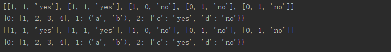
如果想要保存一些结果或者数据以方便后续使用，Python 中的 pickle 模块非常有 用。pickle 模块可以接受几乎所有的 Python 对象，并且将其转换成字符串表示，该 过程叫做封装（pickling）。从字符串表示中重构该对象，称为拆封（unpickling）。 这些字符串表示可以方便地存储和传输。

编写代码：

# coding:utf-8
# pickle模块主要函数的应用举例
import pickle

dataList = [[1, 1, 'yes'],
            [1, 1, 'yes'],
            [1, 0, 'no'],
            [0, 1, 'no'],
            [0, 1, 'no']]
dataDic = {0: [1, 2, 3, 4],
           1: ('a', 'b'),
           2: {'c': 'yes', 'd': 'no'}}

# 使用dump()将数据序列化到文件中
fw = open('dataFile.txt', 'wb')
# Pickle the list using the highest protocol available.
pickle.dump(dataList, fw, -1)
# Pickle dictionary using protocol 0.
pickle.dump(dataDic, fw)
fw.close()

# 使用load()将数据从文件中序列化读出
fr = open('dataFile.txt', 'rb')
data1 = pickle.load(fr)
print(data1)
data2 = pickle.load(fr)
print(data2)
fr.close()

# 使用dumps()和loads()举例
p = pickle.dumps(dataList)
print(pickle.loads(p))
p = pickle.dumps(dataDic)
print(pickle.loads(p))

代码运行效果如下：

（四）SciPy

SciPy（http://scipy.org/） 是建立在NumPy 基础上，用于数值运算的开源工具包。 SciPy 提供很多高效的操作，可以实现数值积分、优化、统计、信号处理，以及对 我们来说最重要的图像处理功能。

4.1 图像模糊

图像的高斯模糊是非常经典的图像卷积例子。本质上，图像模糊就是将（灰度）图 像 I 和一个高斯核进行卷积操作：

其中 * 表示卷积操作；Gσ 是标准差为 σ 的二维高斯核，定义为 :

编写代码：

# -*- coding: utf-8 -*-
from PIL import Image
from pylab import *
from scipy.ndimage import filters

# 添加中文字体支持
from matplotlib.font_manager import FontProperties
font = FontProperties(fname=r"c:\\windows\\fonts\\SimSun.ttc", size=14)

#im = array(Image.open('board.jpeg'))
im = array(Image.open('D:\\Python\\chapterone\\dog3.jpg').convert('L'))

figure()
gray()
axis('off')
subplot(1, 4, 1)
axis('off')
title(u'原图', fontproperties=font)
imshow(im)

for bi, blur in enumerate([2, 5, 10]):
  im2 = zeros(im.shape)
  im2 = filters.gaussian_filter(im, blur)
  im2 = np.uint8(im2)
  imNum=str(blur)
  subplot(1, 4, 2 + bi)
  axis('off')
  title(u'标准差为'+imNum, fontproperties=font)
  imshow(im2)

show()

代码运行效果如下：

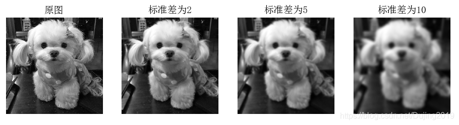
图像显示随着 σ 的增加，一幅图像被模糊的程度。σ 越大，处理后的图像细节丢失越多。如果打算模糊一幅彩色图像，可以对每一个颜色通道进行高斯模糊。

4.2 图像导数

强度的变化可以用灰度图像I（对于彩色图像，通常对每个颜色通道分别计算导数）的x 和 y方向导数 $I_x$ 和 $I_y$ 进行描述。

图像的梯度向量为:

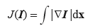
梯度有两个重要的属性，一是梯度的大小：

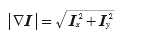
它描述了图像强度变化的强弱，一是梯度的角度：

描述了图像中在每个点（像素）上强度变化最大的方向。NumPy 中的 arctan2() 函数 返回弧度表示的有符号角度，角度的变化区间为 -π…π。

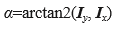
我们可以用离散近似的方式来计算图像的导数。图像导数大多数可以通过卷积简单地实现：

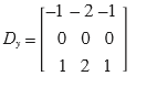
对于 Dx 和 Dy，可以选择 Sobel 滤波器：


编写代码：

# -*- coding: utf-8 -*-
from PIL import Image
from pylab import *
from scipy.ndimage import filters
import numpy

# 添加中文字体支持
from matplotlib.font_manager import FontProperties
font = FontProperties(fname=r"c:\windows\fonts\SimSun.ttc", size=14)

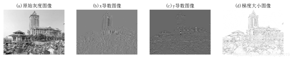
im = array(Image.open('D:\\Python\\chapterone\\jimei2.jpg').convert('L'))
gray()

subplot(1, 4, 1)
axis('off')
title(u'(a)原始灰度图像', fontproperties=font)
imshow(im)

# Sobel derivative filters
imx = zeros(im.shape)
filters.sobel(im, 1, imx)
subplot(1, 4, 2)
axis('off')
title(u'(b)x导数图像', fontproperties=font)
imshow(imx)

imy = zeros(im.shape)
filters.sobel(im, 0, imy)
subplot(1, 4, 3)
axis('off')
title(u'(c)y导数图像', fontproperties=font)
imshow(imy)

#mag = numpy.sqrt(imx**2 + imy**2)
mag = 255-numpy.sqrt(imx**2 + imy**2)
subplot(1, 4, 4)
title(u'(d)梯度大小图像', fontproperties=font)
axis('off')
imshow(mag)

show()

代码运行效果如下：

上述计算图像导数的方法有一些缺陷：在该方法中，滤波器的尺度需要随着图像分 辨率的变化而变化。为了在图像噪声方面更稳健，以及在任意尺度上计算导数，我 们可以使用高斯导数滤波器：

其中，Gσx 和 Gσy 表示 Gσ 在 x 和 y 方向上的导数，Gσ 为标准差为 σ 的高斯函数。

# -*- coding: utf-8 -*-
from PIL import Image
from pylab import *
from scipy.ndimage import filters
import numpy

# 添加中文字体支持
#from matplotlib.font_manager import FontProperties
#font = FontProperties(fname=r"c:\windows\fonts\SimSun.ttc", size=14)

def imx(im, sigma):
    imgx = zeros(im.shape)
    filters.gaussian_filter(im, sigma, (0, 1), imgx)
    return imgx


def imy(im, sigma):
    imgy = zeros(im.shape)
    filters.gaussian_filter(im, sigma, (1, 0), imgy)
    return imgy


def mag(im, sigma):
    # there's also gaussian_gradient_magnitude()
    #mag = numpy.sqrt(imgx**2 + imgy**2)
    imgmag = 255 - numpy.sqrt(imgx ** 2 + imgy ** 2)
    return imgmag


im = array(Image.open('D:\\Python\\chapterone\\jimei2.jpg').convert('L'))
figure()
gray()

sigma = [2, 5, 10]

for i in  sigma:
    subplot(3, 4, 4*(sigma.index(i))+1)
    axis('off')
    imshow(im)
    imgx=imx(im, i)
    subplot(3, 4, 4*(sigma.index(i))+2)
    axis('off')
    imshow(imgx)
    imgy=imy(im, i)
    subplot(3, 4, 4*(sigma.index(i))+3)
    axis('off')
    imshow(imgy)
    imgmag=mag(im, i)
    subplot(3, 4, 4*(sigma.index(i))+4)
    axis('off')
    imshow(imgmag)

show()

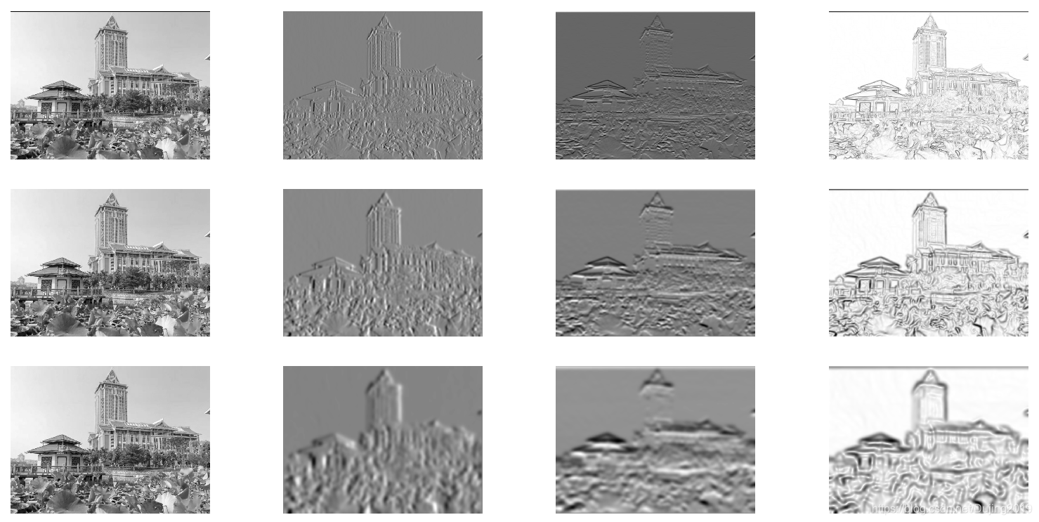
注释：

1. 第一列为原始灰度图像分别使用σ=2 ，σ=5，σ=10的高斯导数滤波器处理后的图像。
2. 第二列为x 导数图像分别使用σ=2 ，σ=5，σ=10的高斯导数滤波器处理后的图像。
3. 第三列为y 导数图像分别使用σ=2 ，σ=5，σ=10的高斯导数滤波器处理后的图像。
4. 第四列为梯度大小图像分别使用σ=2 ，σ=5，σ=10的高斯导数滤波器处理后的图像。

4.3 形态学：对象计数

形态学（或数学形态学）是度量和分析基本形状的图像处理方法的基本框架与集合。 形态学通常用于处理二值图像，但是也能够用于灰度图像。二值图像是指图像的每 个像素只能取两个值，通常是 0 和 1。二值图像通常是，在计算物体的数目，或者度量其大小时，对一幅图像进行阈值化后的结果。

编写代码：

# -*- coding: utf-8 -*-
from PIL import Image
from numpy import *
from scipy.ndimage import measurements, morphology
from pylab import *

"""   This is the morphology counting objects example in Section 1.4.  """

# 添加中文字体支持
from matplotlib.font_manager import FontProperties
font = FontProperties(fname=r"c:\windows\fonts\SimSun.ttc", size=14)

# load image and threshold to make sure it is binary
figure()
gray()
im = array(Image.open('D:\\Python\\chapterone\\8.png').convert('L'))
subplot(221)
imshow(im)
axis('off')
title(u'(a)原始二值图像', fontproperties=font)
im = (im < 128)

labels, nbr_objects = measurements.label(im)
print "Number of objects:", nbr_objects
subplot(222)
imshow(labels)
axis('off')
title(u'(b)原始图像的标签图像', fontproperties=font)

# morphology - opening to separate objects better
im_open = morphology.binary_opening(im, ones((9, 5)), iterations=2)
subplot(223)
imshow(im_open)
axis('off')
title(u'(c)开操作后的二值图像', fontproperties=font)

labels_open, nbr_objects_open = measurements.label(im_open)
print "Number of objects:", nbr_objects_open
subplot(224)
imshow(labels_open)
axis('off')
title(u'(d)开操作后图像的标签图像', fontproperties=font)

show()

代码运行效果如下：

（五）高级示例：图像去噪

图像去噪是在去除图像噪声的同时，尽可能地保留图像细节和结构的处理技术。这里使用ROF （Rudin-Osher-Fatemi）去噪模型。ROF 模型具有很好的性质：使处理后的图像更平滑，同时保持图像边缘和结构信息。

一幅（灰度）图像I 的全变差（Total Variation，TV）定义为梯度范数之和。在连 续表示的情况下，全变差表示为：

在离散表示的情况下，全变差表示为：

其中，上面的式子是在所有图像坐标 x=[x, y] 上取和。

编写代码：

# -*- coding: utf-8 -*-
from pylab import *
from numpy import *
from numpy import random
from scipy.ndimage import filters
from scipy.misc import imsave
from PCV.tools import rof

""" This is the de-noising example using ROF in Section 1.5. """

# 添加中文字体支持
from matplotlib.font_manager import FontProperties
font = FontProperties(fname=r"c:\windows\fonts\SimSun.ttc", size=14)

# create synthetic image with noise
im = zeros((500,500))
im[100:400,100:400] = 128
im[200:300,200:300] = 255
im = im + 30*random.standard_normal((500,500))

U,T = rof.denoise(im,im)
G = filters.gaussian_filter(im,10)


# save the result
#imsave('synth_original.pdf',im)
#imsave('synth_rof.pdf',U)
#imsave('synth_gaussian.pdf',G)


# plot
figure()
gray()

subplot(1,3,1)
imshow(im)
#axis('equal')
axis('off')
title(u'(a)原噪声图像', fontproperties=font)

subplot(1,3,2)
imshow(G)
#axis('equal')
axis('off')
title(u'(b)高斯模糊后的图像', fontproperties=font)

subplot(1,3,3)
imshow(U)
#axis('equal')
axis('off')
title(u'(c)ROF降噪后的图像', fontproperties=font)

show()

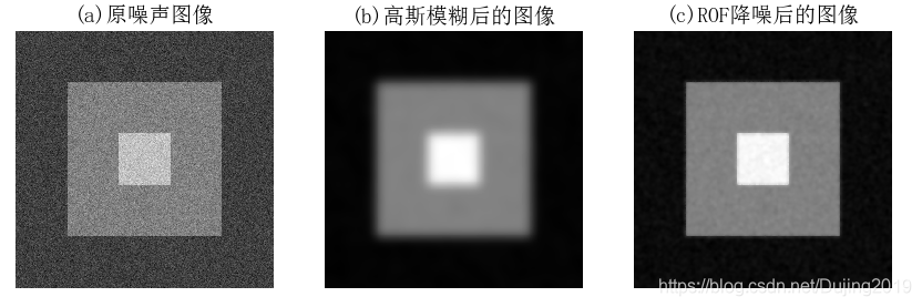
正如所看到的，ROF 算法去噪后的图像很好地保留了图像的边缘信息。下面看一下在实际图像中使用 ROF 模型去噪的效果：

编写代码：

# -*- coding: utf-8 -*-
from PIL import Image
from pylab import *
from numpy import *
from numpy import random
from scipy.ndimage import filters
from scipy.misc import imsave
from PCV.tools import rof

""" This is the de-noising example using ROF in Section 1.5. """

# 添加中文字体支持
from matplotlib.font_manager import FontProperties
font = FontProperties(fname=r"c:\windows\fonts\SimSun.ttc", size=14)

im = array(Image.open('D:\\Python\\chapterone\\noise.png').convert('L'))

U,T = rof.denoise(im,im)
G = filters.gaussian_filter(im,10)


# save the result
#imsave('synth_original.pdf',im)
#imsave('synth_rof.pdf',U)
#imsave('synth_gaussian.pdf',G)


# plot
figure()
gray()

subplot(1,3,1)
imshow(im)
#axis('equal')
axis('off')
title(u'(a)原噪声图像', fontproperties=font)

subplot(1,3,2)
imshow(G)
#axis('equal')
axis('off')
title(u'(b)高斯模糊后的图像', fontproperties=font)

subplot(1,3,3)
imshow(U)
#axis('equal')
axis('off')
title(u'(c)ROF降噪后的图像', fontproperties=font)

show()

代码运行效果如下：

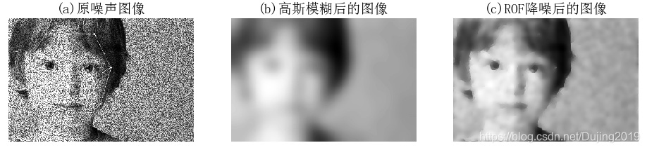
经过 ROF 去噪后的图像如上图所示。为了方便比较，该图中同样显示了模糊后的图像。可以看到，ROF 去噪后的图像保留了边缘和图像的结构信息，同时模糊了 “噪声”。