计算机视觉——基本的图像操作和处理（python）

1.1 PIL：Python图像处理类库

PIL（Python Imaging Library Python，图像处理类库）提供了通用的图像处理功能，以及大量有用的基本图像操作，比如图像缩放、裁剪、旋转、颜色转换等。
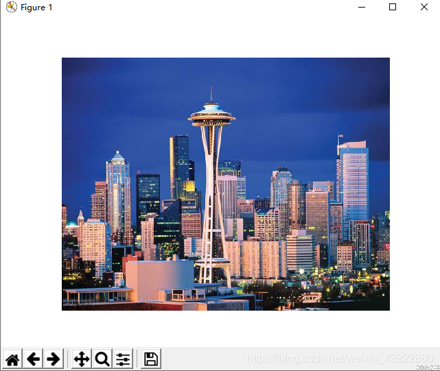
图像的读取和显示

from PIL import Image
import matplotlib.pyplot as plt #使用 matplotlib 来显示图片，可以让图片显示到jupyter的页面
pil_im = Image.open('123.jpg') 
plt.axis('off') #取消显示横纵坐标
plt.imshow(pil_im)  
plt.show()  #显示打开的图片

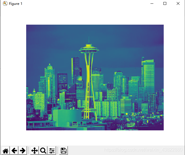
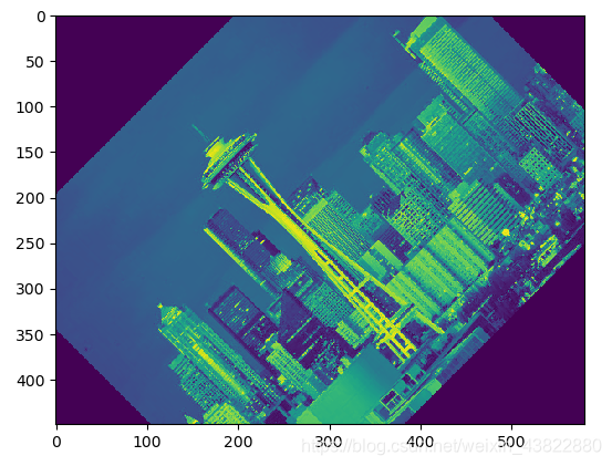
图像的灰度图显示
使用 convert() 方法来实现。

from PIL import Image
import matplotlib.pyplot as plt #使用 matplotlib 来显示图片，可以让图片显示到jupyter的页面
pil_im = Image.open('123.jpg').convert('L')
plt.axis('off') #取消显示横纵坐标
plt.imshow(pil_im)  
plt.show()  #显示打开的图片

1.1.1转换图像格式

1.1.2创建缩略图

创建最长边为 50(横)40(纵)像素的缩略图
ps:为了方便看像素所以加上了横纵坐标

pil_im.thumbnail((50,40))

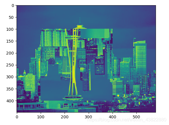
1.1.3复制和粘贴图像区域

crop() 方法：从一幅图像中裁剪指定区域：
box = (100,100,400,400)
region = pil_im.crop(box)
该区域用四元组来指定。四元组的坐标依次是（左，上，右，下）。PIL 中指定坐标系的左上角坐标为（0，0）。可以旋转上面代码中获取的区域。
paste() 方法:将该区域放回去。
具体实现如下：

from PIL import Image
import matplotlib.pyplot as plt #使用 matplotlib 来显示图片，可以让图片显示到jupyter的页面
pil_im = Image.open('123.jpg').convert('L')
box = (100,100,400,400)
region = pil_im.crop(box)
region = region.transpose(Image.ROTATE_180)
pil_im.paste(region,box)
plt.imshow(pil_im)  
plt.show()  #显示打开的图片

1.1.4调整尺寸和旋转

resize() 方法:该方法的参数是一个元组，用来指定新图像的大小
rotate() 方法:逆时针方式表示旋转角度

out = pil_im.resize((128,128))
out = pil_im.rotate(45)

1.2 Matplotlib

处理数学运算、绘制图表，或者在图像上绘制点、直线和曲线时,Matplotlib是个很好的类库，具有比 PIL 更强大的绘图功能。

1.2.1绘制图像、点和线

from PIL import Image
from pylab import *
# 读取图像到数组中
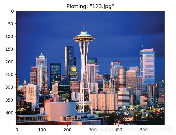
im = array(Image.open('123.jpg'))
# 绘制图像
imshow(im)
# 一些点
x = [100,100,400,400]
y = [200,300,200,300]
# 使用红色星状标记绘制点
plot(x,y,'r*')
# 绘制连接前两个点的线 为黑色
plot(x[:2],y[:2],'k')
# 添加标题，显示绘制的图像
title('Plotting: "123.jpg"')
show()

1.2.2图像轮廓和直方图

绘制轮廓需要对每个坐标 [x, y] 的像素值施加同一个阈值，所以首先需要将图像灰度化后，再用hist() 函数绘制直方图：
flatten() 方法：将任意数组按照行优先准则转换成一维数组。

from PIL import Image
from pylab import *
# 读取图像到数组中
im = array(Image.open('123.jpg').convert('L'))
# 新建一个图像
figure(1)
# 不使用颜色信息
gray()
# 在原点的左上角显示轮廓图像
contour(im, origin='image')
axis('equal')
axis('off')
figure(2)
hist(im.flatten(),128)
show()

1.2.3交互式标注

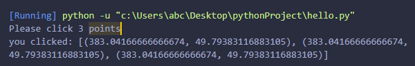
ginput() 函数:单机指定次数后，程序将这些点击的坐标 [x, y] 自动保存在 x 列表里

from PIL import Image
from pylab import *
im = array(Image.open('123.jpg'))
imshow(im)
print('Please click 3 points')
x = ginput(3)
print('you clicked:',x)
show()

1.3 NumPy

NumPy：非常有名的 Python 科学计算工具包，其中包含了大量有用的思想，比如数组对象（用来表示向量、矩阵、图像等）以及线性代数函数。

1.3.1图像数组表示

array() 方法：将图像转换成 NumPy 的数组对象

from PIL import Image
from pylab import *
im = array(Image.open('123.jpg'))
print(im.shape, im.dtype)
im = array(Image.open('123.jpg').convert('L'),'f')
print(im.shape, im.dtype)

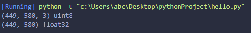
小结：
1.(449，580，3)表示图片表示为数组大小有449行580列，3个颜色通道，为unit8的数据类型（无符号八位整数）
2.（449，580)为对图像进行灰度化处理，并且疆数据类型设置为浮点型后，图片表示为数组大小有449行580列，灰度图像没有颜色信息，所以在形状元组中，它只有两个数值。

1.3.2灰度变换

from PIL import Image
from numpy import *
import matplotlib.pyplot as plt 
im = array(Image.open('123.jpg').convert('L'))
im2 = 255 - im # 对图像进行反相处理
im3 = (100.0/255) * im + 100 # 将图像像素值变换到 100...200 区间
im4 = 255.0 * (im/255.0)**2 # 对图像像素值求平方后得到的图像
#创建新的figure
fig = plt.figure()
#必须通过add_subplot()创建一个或多个绘图
#ax = fig.add_subplot(221)
#绘制2x2两行两列共四个图，编号从1开始
ax1 = fig.add_subplot(221)
ax1.imshow(im)
ax2 = fig.add_subplot(222) 
ax2.imshow(im2)
ax3 = fig.add_subplot(223)
ax3.imshow(im3)
ax4 = fig.add_subplot(224)
ax4.imshow(im4)
#图片的显示
plt.show()
print(int(im.min()), int(im.max()))
print(int(im2.min()),int(im2.max()))
print(int(im3.min()),int(im3.max()))
print(int(im4.min()),int(im4.max()))

小结：
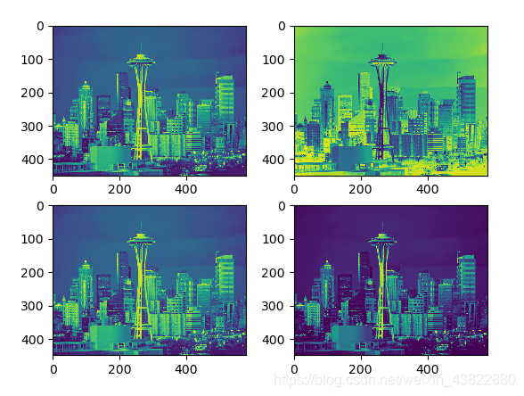
1.图一为灰度图像
2.图二将灰度图像进行反相处理
3.图三将图像的像素值变换到 100…200区间
4.图四对图像使用二次函数变换，使较暗的像素值变得更小。
5.0，254表示图一像中最小像素值为0，最大像素值为254（后三组同理）

1.3.3图像缩放

先将图像缩放写成自定义的简单函数，之后会用到

from PIL import Image
from numpy import *
import matplotlib.pyplot as plt 
def imresize(im,sz):
 """ 使用 PIL 对象重新定义图像数组的大小 """
 pil_im = Image.fromarray(uint8(im))
 return array(pil_im.resize(sz))

1.3.4直方图均衡化

直方图均衡化:指将一幅图像的灰度直方图变平，使变换后的图像中每个灰度值的分布概率都相同。直方图均衡化通常是对图像灰度值进行归一化的一个非常好的方法，并且可以增强图像的对比度。

from PIL import Image
from pylab import *
from numpy import *
import matplotlib.pyplot as plt 
def histeq(im,nbr_bins = 256):
    """对一幅灰度图像进行直方图均衡化"""
    #计算图像的直方图
    #在numpy中，也提供了一个计算直方图的函数histogram(),第一个返回的是直方图的统计量，第二个为每个bins的中间值
    imhist,bins = histogram(im.flatten(),nbr_bins,normed= True)
    cdf = imhist.cumsum()   #
    cdf = 255.0 * cdf / cdf[-1]
    #使用累积分布函数的线性插值，计算新的像素值
    im2 = interp(im.flatten(),bins[:-1],cdf)
    return im2.reshape(im.shape),cdf


im = array(Image.open('123.jpg').convert('L'))
#figure()
#hist(im.flatten(),256)

im2,cdf = histeq(im)
#figure()
#ist(im2.flatten(),256)
#show()

fig = plt.figure()
#必须通过add_subplot()创建一个或多个绘图
#ax = fig.add_subplot(221)
#绘制2x2两行两列共四个图，编号从1开始
ax1 = fig.add_subplot(221)
ax1.imshow(im)
ax2 = fig.add_subplot(222) 
ax2.imshow(im2)
ax3 = fig.add_subplot(223)
ax3=hist(im.flatten(),256)
ax4 = fig.add_subplot(224)
ax4=hist(im2.flatten(),256)
#图片的显示
plt.show()

小结：
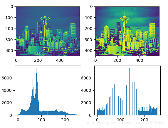
1.图像结果依次为原图与其直方图和均衡化后的图像与其直方图
2.从图像来看，均衡化后色彩的对比度更为明显
3.从直方图来看，均衡化后灰度值分布的概率比之前平均了

1.3.5图像平均

图像平均：减少图像噪声的一种简单方式，通常用于艺术特效。
mean() ：计算平均图像

def compute_average(imlist): 
 """ 计算图像列表的平均图像 """
 # 打开第一幅图像，将其存储在浮点型数组中
 averageim = array(Image.open(imlist[0]), 'f')
 for imname in imlist[1:]:
 try:
 averageim += array(Image.open(imname))
 except:
 print imname + '...skipped'
 averageim /= len(imlist)
 # 返回 uint8 类型的平均图像
 return array(averageim, 'uint8')

1.3.6图像的主成分分析（PCA）

PCA（Principal Component Analysis，主成分分析）：一个非常有用的降维技巧。

1.3.7使用pickle模块

1.4 SciPy

SciPy：建立在 NumPy 基础上，用于数值运算的开源工具包。SciPy 提供很多高效的操作，可以实现数值积分、优化、统计、信号处理，以及对我们来说最重要的图像处理功能。

1.4.1图像模糊

本质上，图像模糊就是将（灰度）图像 I 和一个高斯核进行卷积操作。高斯模糊通常是其他图像处理操作的一部分，比如图像插值操作、兴趣点计算以及很多其他应用。

from PIL import Image
from numpy import *
from scipy.ndimage import filters
import matplotlib.pyplot as plt #使用 matplotlib 来显示图片，可以让图片显示到jupyter的页面
im = array(Image.open('123.jpg').convert('L'))
im2 = filters.gaussian_filter(im,2)
im3 = filters.gaussian_filter(im,5)
fig = plt.figure()
ax1 = fig.add_subplot(131)
ax1.imshow(im)
ax2 = fig.add_subplot(132) 
ax2.imshow(im2)
ax3 = fig.add_subplot(133) 
ax3.imshow(im3)
plt.show()

1. filters.gaussian_filter(im,5)中，5表示σ 值。结果中图片分别为原图，σ=2的高斯滤波器，σ =5的高斯滤波器，高斯模糊的情况。
2. 可见随着 σ 的增加，一幅图像被模糊的程度。σ 越大处理后的图像细节丢失越多。

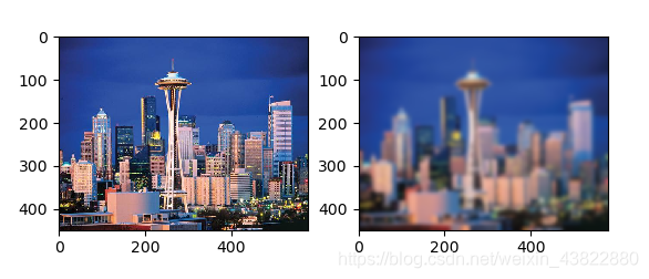
如果打算模糊一幅彩色图像，只需简单地对每一个颜色通道进行高斯模糊

from PIL import Image
from numpy import *
from scipy.ndimage import filters
import matplotlib.pyplot as plt #使用 matplotlib 来显示图片，可以让图片显示到jupyter的页面
im = array(Image.open('123.jpg'))
im2 = zeros(im.shape)
for i in range(3):
 im2[:,:,i] = filters.gaussian_filter(im[:,:,i],5) 
im2 = uint8(im2)
fig = plt.figure()
ax1 = fig.add_subplot(121)
ax1.imshow(im)
ax2 = fig.add_subplot(122) 
ax2.imshow(im2)
plt.show()