本文通过TensorFlow构建深度神经网络对MNIST手写体数字进行识别。学习其他内容参考TensorFlow 学习目录。
目录
一、MNIST数据集
链接:https://pan.baidu.com/s/1pX272g5fKo6zzc0SIuLB9w
提取码:kj9m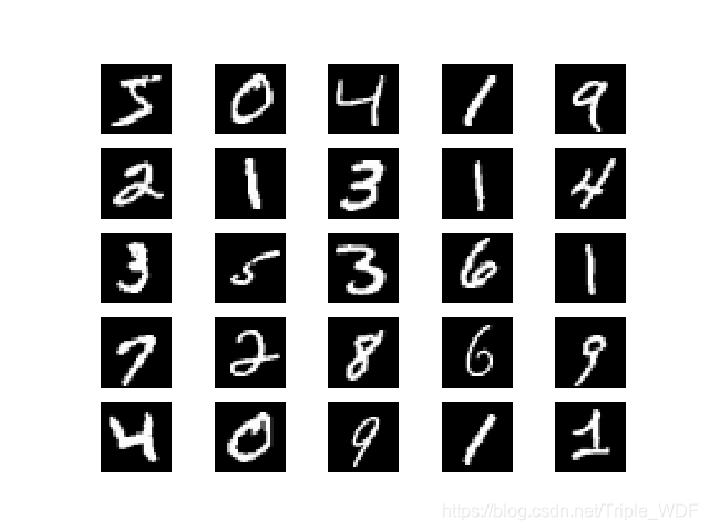
该数据集有60000个训练集,10000个测试集,数字有0~9十个数字。图片格式是灰度图,28*28大小,pkl中存储的形式是50000*784,10000*784,以及对应的标签。
<1>通过如下代码对数据集进行加载
# .py file: mnist_loader.py
import pickle
import gzip
import numpy as np

def load_data():
    f = gzip.open('D:\dataset\mnist.pkl.gz', 'rb')
    training_data, validation_data, test_data = pickle.load(f, encoding='bytes')
    # print (training_data)
    # print (validation_data)
    # print (test_data)
    f.close()
    return (training_data, validation_data, test_data)

def vectorized_result(j):
    e = np.zeros((10, 1))
    e[j] = 1.0
    return e

def load_data_wrapper():
    tr_d, va_d, te_d = load_data()
    #training_data
    training_inputs = [np.reshape(x, (784, 1)) for x in tr_d[0]]
    training_results = [vectorized_result(y) for y in tr_d[1]]
    training_data = zip(training_inputs, training_results)

    #validation_data
    validation_inputs = [np.reshape(x, (784, 1)) for x in va_d[0]]
    validation_results = [vectorized_result(y) for y in va_d[1]]
    validation_data = zip(validation_inputs, validation_results)

    #test_data
    test_inputs = [np.reshape(x, (784, 1)) for x in te_d[0]]
    test_data = zip(test_inputs, te_d[1])

    return (training_data, validation_data, test_data)
<2>通过如下代码对数据集进行划分,将validation的10000个样例划分到训练集中,这样训练集就有60000张图片。
# .py file: get_Dataset.py

import numpy as np
import mnist_loader

def get_Dataset(name='mnist'):
    if name == 'mnist':
        t, v, tt = mnist_loader.load_data_wrapper()
        validation_data = list(v)
        training_data = list(t) + validation_data
        testing_data = list(tt)

        len_t = len(training_data)
        len_tdi = len(training_data[0][0])
        len_tl = len(training_data[0][1])
        x_train = np.zeros((len_t, len_tdi))
        y_train = np.zeros((len_t, len_tl))
        for i in range(len_t):
            x_train[i] = np.array(training_data[i][0]).transpose()
            y_train[i] = np.array(training_data[i][1]).transpose()

        len_tt = len(testing_data)
        x_test = np.zeros((len_tt, len_tdi))
        y_test = np.zeros(len_tt)
        for i in range(len_tt):
            x_test[i] = np.array(testing_data[i][0]).transpose()
            y_test[i] = testing_data[i][1]
        return x_train, y_train, x_test, y_test
二、构建深度神经网络
<1>入口 placeholder
inputs = tf.placeholder(dtype=tf.float32, shape=[None, 784], name='inputs')
labels = tf.placeholder(dtype=tf.float32, shape=[None, 10], name='labels')
predict_labels = tf.placeholder(dtype=tf.int64, shape=[None], name='predict_labels')
其中inputs表示输入的784维度的灰度图的向量拉伸,labels是一个one-hot向量,predict_labels不是one-hot向量,是直接的0~9数字。
<2>卷积层定义
def conv2d(x, id, filter_size):
    with tf.variable_scope('conv2d_'+str(id)):
        w = tf.get_variable(name='filter', initializer=tf.truncated_normal(shape=filter_size, stddev=0.1), dtype=tf.float32)
        b = tf.get_variable(name='bias', initializer=tf.constant(0.1, shape=[filter_size[3]], dtype=tf.float32))
        z = tf.nn.relu(tf.nn.conv2d(x, w, strides=[1, 1, 1, 1], padding='SAME') + b)
return z这里用到了tf.variable_scope()+tf.get_variable()的方式,具体参考TensorFlow 共享变量。
<3>池化层定义,此处采用最大值池化
def pooling(x):
    return tf.nn.max_pool(x, ksize=[1, 2, 2, 1], strides=[1, 2, 2, 1], padding='SAME')
<4>Tensor拉伸操作,flatten操作:将多通道的tensor转化为一维向量
def flatten(x):
    l = x.get_shape()[1:]
    length = l[1]*l[2]*l[0]
    x = tf.reshape(x, shape=[-1, length])
    return x
<5>全连接层
def fully(x, id, neurons):
    with tf.variable_scope('fully'+str(id)):
        L = int(x.get_shape()[1])
        w = tf.get_variable(name='w', initializer=tf.truncated_normal(shape=[L, neurons], stddev=0.1), dtype=tf.float32)
        b = tf.get_variable(name='b', initializer=tf.constant(0.1, shape=[neurons], dtype=tf.float32))
        z = tf.nn.relu(tf.nn.xw_plus_b(x, w, b))
    return z
三、网络结构的设计
- 图像输入[batchsize, 784]
- net为图像reshape之后的结果,[batchsize, 28, 28, 1],因为是灰度图,所以通道数为 1。
- 建立一个大小为5*5,进入通道数为 1,输出通道数为64的卷积核对net进行卷积操作
- 对net进行一次2*2大小的池化操作
- 建立一个大小为3*3,计入通道数为 64,输出通道数为64的卷积核对net进行卷积操作
- 对net进行一次2*2大小的池化操作
- 将net进行拉伸,变为一维向量(加上batchsize其实是二维)
- 加入一层神经元个数为512的全连接层
- 加入一层神经元个数为10的全连接层作为输出层
net = tf.reshape(inputs, shape=[-1, 28, 28, 1])
net = conv2d(net, 1, [5, 5, 1, 64])
net = pooling(net)
net = conv2d(net, 2, [3, 3, 64, 64])
net = pooling(net)
net = flatten(net)

net = fully(net, 3, 512)
logits = fully(net, 4, 10)
四、定义损失函数,以及优化方式
采用交叉熵作为损失函数,采用AdamOptimizer作为优化方式。
loss = tf.reduce_mean(tf.nn.softmax_cross_entropy_with_logits(labels=labels, logits=logits))
train_step = tf.train.AdamOptimizer(1e-4).minimize(loss)
五、预测
correct_prediction = tf.equal(tf.argmax(logits, 1), predict_labels)
accuracy = tf.reduce_mean(tf.cast(correct_prediction, tf.float32))
六、定义Epochs、batch_size进行训练
epochs = 100
batch_size = 32

with tf.Session(config=tf.ConfigProto(allow_soft_placement=True)) as sess:
    sess.run(tf.global_variables_initializer())
    for epoch in range(epochs):
        for batch in range(int(x_train.shape[0]/batch_size)):
            batch_xs = x_train[batch*batch_size: (batch+1)*batch_size]
            batch_ys = y_train[batch*batch_size: (batch+1)*batch_size]
            feed_dict = {
                inputs: batch_xs,
                labels: batch_ys
            }
            sess.run(train_step, feed_dict=feed_dict)
        acc = sess.run(accuracy, feed_dict={inputs: x_test, predict_labels: y_test})
        print ("Epoch ", epoch+1, " acc=", acc*100, "%")
输出结果
Epoch  1  acc= 28.949999809265137 %
Epoch  2  acc= 57.270002365112305 %
Epoch  3  acc= 57.74000287055969 %
Epoch  4  acc= 57.88000226020813 %
Epoch  5  acc= 67.66999959945679 %
Epoch  6  acc= 77.30000019073486 %
Epoch  7  acc= 87.48999834060669 %
Epoch  8  acc= 87.58999705314636 %
Epoch  9  acc= 87.6200020313263 %
Epoch  10  acc= 87.61000037193298 %
Epoch  11  acc= 87.58000135421753 %
Epoch  12  acc= 87.80999779701233 %
Epoch  13  acc= 87.77999877929688 %
Epoch  14  acc= 87.87000179290771 %
Epoch  15  acc= 87.84000277519226 %
Epoch  16  acc= 87.8000020980835 %
Epoch  17  acc= 87.73999810218811 %
Epoch  18  acc= 87.76999711990356 %
Epoch  19  acc= 87.77999877929688 %
Epoch  20  acc= 87.87000179290771 %
Epoch  21  acc= 87.84000277519226 %
Epoch  22  acc= 87.80999779701233 %
Epoch  23  acc= 87.69000172615051 %
Epoch  24  acc= 87.74999976158142 %
Epoch  25  acc= 87.80999779701233 %
Epoch  26  acc= 98.86999726295471 %
Epoch  27  acc= 99.16999936103821 %
Epoch  28  acc= 99.19000267982483 %
Epoch  29  acc= 99.1599977016449 %
Epoch  30  acc= 99.15000200271606 %
Epoch  31  acc= 99.08000230789185 %
Epoch  32  acc= 99.14000034332275 %
Epoch  33  acc= 99.16999936103821 %
Epoch  34  acc= 99.1599977016449 %
Epoch  35  acc= 99.14000034332275 %
Epoch  36  acc= 99.04999732971191 %
Epoch  37  acc= 99.18000102043152 %
Epoch  38  acc= 99.22000169754028 %
Epoch  39  acc= 99.19000267982483 %
Epoch  40  acc= 99.19999837875366 %
Epoch  41  acc= 99.26999807357788 %
Epoch  42  acc= 99.11999702453613 %
Epoch  43  acc= 99.22000169754028 %
Epoch  44  acc= 99.19999837875366 %
Epoch  45  acc= 99.26999807357788 %
Epoch  46  acc= 99.26999807357788 %
Epoch  47  acc= 99.09999966621399 %
Epoch  48  acc= 99.1100013256073 %
Epoch  49  acc= 99.14000034332275 %
Epoch  50  acc= 99.01999831199646 %
Epoch  51  acc= 99.12999868392944 %
Epoch  52  acc= 98.96000027656555 %
Epoch  53  acc= 99.11999702453613 %
Epoch  54  acc= 99.11999702453613 %
Epoch  55  acc= 99.22999739646912 %
Epoch  56  acc= 99.26000237464905 %
Epoch  57  acc= 99.25000071525574 %
Epoch  58  acc= 99.23999905586243 %
Epoch  59  acc= 99.19000267982483 %
Epoch  60  acc= 99.21000003814697 %
Epoch  61  acc= 99.23999905586243 %
Epoch  62  acc= 99.25000071525574 %
Epoch  63  acc= 99.19000267982483 %
Epoch  64  acc= 99.16999936103821 %
Epoch  65  acc= 99.04000163078308 %
Epoch  66  acc= 99.12999868392944 %
Epoch  67  acc= 99.1100013256073 %
Epoch  68  acc= 99.22000169754028 %
Epoch  69  acc= 99.18000102043152 %
Epoch  70  acc= 99.22000169754028 %
Epoch  71  acc= 99.04000163078308 %
Epoch  72  acc= 99.22000169754028 %
Epoch  73  acc= 99.23999905586243 %
Epoch  74  acc= 99.26999807357788 %
Epoch  75  acc= 99.05999898910522 %
Epoch  76  acc= 99.19000267982483 %
Epoch  77  acc= 99.21000003814697 %
Epoch  78  acc= 99.19999837875366 %
Epoch  79  acc= 99.22000169754028 %
Epoch  80  acc= 99.23999905586243 %
Epoch  81  acc= 99.15000200271606 %
Epoch  82  acc= 99.25000071525574 %
Epoch  83  acc= 99.25000071525574 %
Epoch  84  acc= 99.1599977016449 %
Epoch  85  acc= 99.22999739646912 %
Epoch  86  acc= 99.21000003814697 %
Epoch  87  acc= 99.2900013923645 %
Epoch  88  acc= 99.21000003814697 %
Epoch  89  acc= 99.27999973297119 %
Epoch  90  acc= 99.18000102043152 %
Epoch  91  acc= 99.04000163078308 %
Epoch  92  acc= 99.26999807357788 %
Epoch  93  acc= 99.12999868392944 %
Epoch  94  acc= 99.2900013923645 %
Epoch  95  acc= 99.32000041007996 %
Epoch  96  acc= 99.25000071525574 %
Epoch  97  acc= 99.2900013923645 %
Epoch  98  acc= 99.26000237464905 %
Epoch  99  acc= 99.16999936103821 %
Epoch  100  acc= 99.27999973297119 %
七、附件:完整代码
import tensorflow as tf
import numpy as np
import get_Dataset

x_train, y_train, x_test, y_test = get_Dataset.get_Dataset(name='mnist')

def conv2d(x, id, filter_size):
    with tf.variable_scope('conv2d_'+str(id)):
        w = tf.get_variable(name='filter', initializer=tf.truncated_normal(shape=filter_size, stddev=0.1), dtype=tf.float32)
        b = tf.get_variable(name='bias', initializer=tf.constant(0.1, shape=[filter_size[3]], dtype=tf.float32))
        z = tf.nn.relu(tf.nn.conv2d(x, w, strides=[1, 1, 1, 1], padding='SAME') + b)
    return z

def pooling(x):
    return tf.nn.max_pool(x, ksize=[1, 2, 2, 1], strides=[1, 2, 2, 1], padding='SAME')

def flatten(x):
    l = x.get_shape()[1:]
    length = l[1]*l[2]*l[0]
    x = tf.reshape(x, shape=[-1, length])
    return x

def fully(x, id, neurons):
    with tf.variable_scope('fully'+str(id)):
        L = int(x.get_shape()[1])
        w = tf.get_variable(name='w', initializer=tf.truncated_normal(shape=[L, neurons], stddev=0.1), dtype=tf.float32)
        b = tf.get_variable(name='b', initializer=tf.constant(0.1, shape=[neurons], dtype=tf.float32))
        z = tf.nn.relu(tf.nn.xw_plus_b(x, w, b))
    return z

inputs = tf.placeholder(dtype=tf.float32, shape=[None, 784], name='inputs')
labels = tf.placeholder(dtype=tf.float32, shape=[None, 10], name='labels')
predict_labels = tf.placeholder(dtype=tf.int64, shape=[None], name='predict_labels')

net = tf.reshape(inputs, shape=[-1, 28, 28, 1])
net = conv2d(net, 1, [5, 5, 1, 64])
net = pooling(net)
net = conv2d(net, 2, [3, 3, 64, 64])
net = pooling(net)
net = flatten(net)

net = fully(net, 3, 512)
logits = fully(net, 4, 10)

loss = tf.reduce_mean(tf.nn.softmax_cross_entropy_with_logits(labels=labels, logits=logits))
train_step = tf.train.AdamOptimizer(1e-4).minimize(loss)

correct_prediction = tf.equal(tf.argmax(logits, 1), predict_labels)
accuracy = tf.reduce_mean(tf.cast(correct_prediction, tf.float32))

epochs = 100
batch_size = 32

with tf.Session(config=tf.ConfigProto(allow_soft_placement=True)) as sess:
    sess.run(tf.global_variables_initializer())
    for epoch in range(epochs):
        for batch in range(int(x_train.shape[0]/batch_size)):
            batch_xs = x_train[batch*batch_size: (batch+1)*batch_size]
            batch_ys = y_train[batch*batch_size: (batch+1)*batch_size]
            feed_dict = {
                inputs: batch_xs,
                labels: batch_ys
            }
            sess.run(train_step, feed_dict=feed_dict)
        acc = sess.run(accuracy, feed_dict={inputs: x_test, predict_labels: y_test})
        print ("Epoch ", epoch+1, " acc=", acc*100, "%")