深度学习---梯度下降&反向传播

梯度下降

对模型进行训练最常用的一种算法


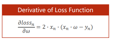
对误差函数进行求导，来不断更新权重W，最终是误差达到最小值。
我们可以看出，梯度下降是是当前最优的解（局部最优解），有点类似于贪心法，

如图所示，我们最终的解是那个红色的点，而不是右侧的最优解。
同时，在梯度下降中遇到的另外一个问题是会遇到梯度为0 的点，此时，梯度下载就不能继续迭代了

化简得

#梯度下降

import numpy as np 
import matplotlib.pyplot as plt 

w=1.0

x_data=[1.0,2.0,3.0]
y_data=[2.0,4.0,6.0]

def function(x):
	return x*w 

def loss(x,y):
	cost=0
	for x_da,y_da in zip(x,y):
		y_pre=function(x_da)
		cost+=(y_pre-y_da)*(y_pre-y_da)
	return cost/len(x)

def gradient(x,y):
	grad=0.0
	for x_da,y_da in zip(x,y):
		grad+=2.0*x_da*(x_da*w-y_da)
	return grad/len(x)

a=0.01#学习率
w_list=[]
loss_list=[]

for i in range(100):
	loss_p=loss(x_data,y_data)
	loss_list.append(loss_p)
	grad_p=gradient(x_data,y_data)
	w-=a*grad_p
	print("loss: ",loss_p)
	print("w: ",w)

plt.plot(np.arange(100),loss_list)
plt.ylabel("cost")
plt.xlabel("count")
plt.show()

随机梯度下降：随机的选取单个样本的损失来计算权重

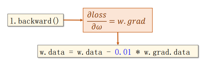
反向传播

面对这复杂的神经网络，怎么去求梯度呢，我们用到了反向传播

反向传播计算过程

#反向传播

#数据样本
x_data=[1.0,2.0,3.0]
y_data=[2.0,4.0,6.0]

#权重
w=torch.Tensor([1.0])#注意要中括号
w.requires_grad=True#需要计算梯度
def function(x):
	return x*w #x会自动进行类型转换成tensor
def loss(x,y):
	y_pre=function(x)
	return (y_pre-y)**2
loss_list=[]

for i in range(100):
	for x_da,y_da in zip(x_data,y_data):
		l=loss(x_da,y_da)
		l.backward()#进行反向传播，求解梯度，并存到w里
		
		w.data=w.data-0.01*w.grad.data
		w.grad.data.zero_()#把梯度数据清零
	loss_list.append(l.item())
	print("progress: ",i,"损失值：",l.item())#取出损失值
print(4,function(4).item())#输出预测后的值
plt.plot(np.arange(100),loss_list)
plt.ylabel("cost")
plt.xlabel("epoch")
plt.show()

在深度学习里，Tensor实际上就是一个多维数组

Reference

《PyTorch深度学习实践》
https://www.bilibili.com/video/BV1Y7411d7Ys?p=5

未完待续…