LSTM-Attention模型：Effective Approaches to Attention-based Neural Machine Translation

参考链接

• 论文链接：https://arxiv.org/pdf/1508.04025v5.pdf
• 项目链接： https://github.com/pytorch/fairseq

模型(model)：

【1】Neural Machine Translation(NMT):

• 神经机器翻译(NMT)是直接用神经网络去模拟条件概率： $p(x|y)$
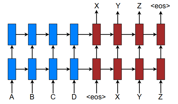
• NMT一般由两个部分组成： $encoder＋decoder$， $encoder$部分读入源句子输出该句子的表示 (representation $S$), $decoder$部分接受 $encoder$部分的输出+ $decoder$已经输出的目标词作为输入并输出一个目标词。因此条件概率可以分解为： $logp(y|x) = \sum_{x=1}^mlogp (y_j|y_{<j},s)$
• 用 $decoder$去模拟该条件概率，因此可以进一步写作： $logp(y|x)=softmax(g(h_j))$ $g$函数的输出向量的维数=词汇表的大小； $h_j$是RNN隐藏状态向量，其公式如下： $h_j = f(h_{j−1}, s)$ $f$是RNN的单元可以是：标准的RNN单元、GRU单元和LSTM单元。
• 模型图：
  
• 这篇论文使用的模型是多层的LSTM+Attention机制；损失函数(目标函数)： $J_t =\sum_{(x,y)∈D} − log p(y|x)$ $D$是语料库

【2】Attention-based Models

• 论文中讲了两种模型： $global$ 和 $local$；两个模型图如下：

  

• Global Attention：

  • 模型图正如上图所示现在解释一下里面的变量：
    • $c_t$:上下文向量；生成它是需要考虑 $encoder$的所有隐藏层状态向量 $\overline{h_t}$
    • $a_t$:对其向量(alignment vector);它的长度是可变的，其长度等于源句子的长度，计算公式如下： $a_t(s)=align(h_t,\overline{h_s})=\frac{exp(socre(h_t,\overline{h}_s))}{\sum_{s'}exp(score(h_t,\overline{h_{s'}}))}$ $score$函数有三种形式： $socre(h_t,\overline{h}_s))= \begin{cases} h_t^T\overline{h_s} \qquad &dot \\ h_t^TW_a\overline{h_s} \qquad & general \\ h_a^Ttanh(W_a[h_t;\overline{h_s}]) \qquad & concat \end{cases}$

• 对于每个输入词 $\overline{w}_s$经过 $encoder$都会产一个隐藏状态向量 $\overline{h}_s$,当 $decoder$在翻译第 $t$个词 $w_t$时, $decoder$先产生当前的隐藏状态向量 $h_t$,然后根据 $a_t(s)$公式，为每个输入词 $\overline{w}_s$计算出一个权值 $a_s$(实数)，所有输入词的权值拼接成一个向量 $a$;即对齐向量(alignment vector)；这也是为啥对齐向量长度为什么等于源句子长度的原因。对其向量的本质就是每个输入词的权重，这样我们根据该权重向量将输入词的隐藏状态向量 $\overline{h}_s$进行加权平均得到上下文向量 $C_t$

• 注意： 模型是使用多层的LSTM网络，上面所用的隐藏状态向量都是最顶层的LSTM的隐藏状态向量。

• Local Attention：

  • $Local Attention$:选择性地关注输入句子中的一小窗口；这样可以减少计算量。
  • 第一步：在原句子中找到一个关注中心点 $p_t$，
  • 第二步：确定关注区间 $[p_t-D,p_t+D]$；D是事先被设置的常数。
  • 第三步：按照 $Global Attention$同样方法计算对其向量 $a$和上下文向量 $c_t$,区别在于在 $Local Attention$中只对窗口 $[p_t-D,p_t+D]$中的输入进行计算，而 $Global Attention$对整个输入句子进行计算。由此可知 $Local Attention$对其向量 $a$长度是固定的，其长度为窗口长度 $D+1$.
  • 确定中心点 $p_t$有两种方法：
    • Monotonic alignment (local-m) ：假设输入句子与输入句子单调对齐，直接令 $p_t=t$。
    • Predictive alignment (local-p)：先按照下面公式预测 $p_t$点： $p_t=S*sigmoid(v_p^Ttanh(W_ph_t))$其中 $W_p$和 $v_p$是可学习的参数； $S$是源句子的长度；则 $p_t\in{[0,S]}$是个实数; 这种情况下我们对齐向量 $a$的计算方式也有所不同： $a_t(s) = align(h_t, \overline{h}_s) exp (−\frac{(s-p_t)^2}{2σ^2})$其中 $σ=\frac{D}{2}$； $s$是窗口 $[p_t-S,p_t+S]$内的整数。

• Input-feeding Approach：

  • 模型图：
    
  • Input-feeding Approach 将上一步注意力向量(attentional vectors) $\tilde{h_t}$与当前步的输入进行拼接 $[tilde{h_t};x]$作为当前时刻 $decoder$的输入以产生当前位置的目标词 $y$。
  • 这种做法的效果：
    • 使得当前模型充分考虑以前的对齐选择(alignment choices)。
    • 这使得我们可以创建了一个非常深的网络，并且横跨水平和垂直方向。

• $global$ 和 $local$两个模型的公共部分

  • $GlobalAttention$和 $Local Attention$不同之处在于：上下文向量 $c_t$的生成；其余部分都是相同的。
  • 注意力向量 $\tilde{h}_t$的生成： $\tilde{h}_t = tanh(W_c[c_t; h_t])$相对先将向量 $c_t$和 $h_t$进行拼接，再将其输入到一个全连接的前馈神经网络中产生了注意力向量 $\tilde{h}_t$.
  • 目标词 $y_t$的生成：将 $\tilde{h}_t$输入到softmax层产生当前目标词 $y_t$的条件概率分布: $p(y_t|y_{<t},x)= softmax(W_s\tilde{h}_t)$