深度学习应用9CIFAR图像识别分类-断点续训

1下载数据集

可以从[(https://www.cs.toronto.edu/~kriz/cifar-10-python.tar.gz) 网址下载 ，下载的文件名是cifar-10-python.tar.gz，该先在Jupty代码目录下建立data子目录，然后把下载的数据文件放到data目录

import urllib.request
import os 
import tarfile
import numpy as np
url='https://www.cs.toronto.edu/~kriz/cifar-10-python.tar.gz'
filepath='data/cifar-10-python.tar.gz'
if not os.path.isfile(filepath):
    result=urllib.request.urlretrievel(url,filepath)
    print('downloaded:',result)
else:
    print('Data file already exists.')
# 解压
if not os.path.exists('data/cifar-10-python.tar.gz'):
    tfile=tarfile.open('data/cifar-10-python.tar.gz','r:gz')
    result=tfile.extractall('data/')
    print('Extracted to ./data/cifar-10-batches-py/')
else:
    print('Directory already exists')

2导入数据集

import pickle
def load_Cifar_batch(filename):
    # laod single batch of cifar
    # open with binary
    with open(filename,'rb')as f:
        data_dict=pickle.load(f,encoding='bytes')
        images=data_dict[b'data']
        labels=data_dict[b'labels']
        
        images=images.reshape(10000,3,32,32)
        images=images.transpose(0,2,3,1)
        labels=np.array(labels)
        return images,labels  

def load_CIFAR_data(data_dir):
    """ load all of cifar """
    images_train = []
    labels_train= []
    for b in range(1,6):
        f = os.path.join(data_dir, 'data_batch_%d' % (b, ))
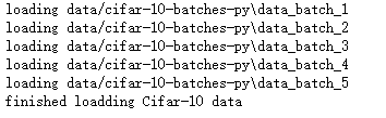
        print('loading',f)
        image_batch,label_batch=load_Cifar_batch(f)
        images_train.append(image_batch)
        labels_train.append(label_batch)
        Xtrain=np.concatenate(images_train)
        Ytrain=np.concatenate(labels_train)
        del image_batch,label_batch
    Xtest,Ytest=load_Cifar_batch(os.path.join(data_dir,'test_batch'))
    print('finished loadding Cifar-10 data')        
    return Xtrain,Ytrain,Xtest,Ytest
data_dir='data/cifar-10-batches-py'
Xtrain,Ytrain,Xtest,Ytest=load_CIFAR_data(data_dir)

输出

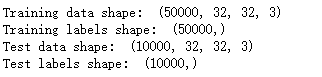
显示数据集维度

print('Training data shape: ', Xtrain.shape)
print('Training labels shape: ', Ytrain.shape)
print('Test data shape: ', Xtest.shape)
print('Test labels shape: ', Ytest.shape)

3显示图像

显示单张图像

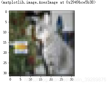
print(Ytrain[6])

输出
2
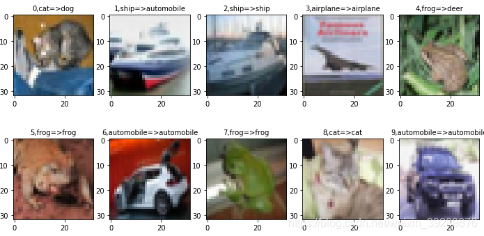
显示多张图像

import matplotlib.pyplot as plt
# 定义标签字典
label_dict={0:'airplane',1:'automobile',2:'bird',3:"cat",4:'deer',5:'dog',6:'frog',7:'house',8:'ship',9:'trunk'}
#定义图像数据及对应标签
def plot_images_labels_prediction(images,labels,prediction,idx,num=10):
    fig=plt.gcf()
    fig.set_size_inches(12,6)
    if num>10:
        num=10
    for i in range(0,num):
        ax=plt.subplot(2,5,1+i)
        ax.imshow(images[idx],cmap='binary')
        title=str(i)+','+label_dict[labels[idx]]
        if len(prediction)>0:
            title+='=>'+label_dict[prediction[idx]]
        ax.set_title(title,fontsize=10)
        idx+=1
    plt.show(0)
plot_images_labels_prediction(Xtest,Ytest,[],1,10)

4数据预处理

4.1图像数据预处理

# 查看数据信息
#第一个像素点
Xtrain[0][0][0]
#第一个像素点在rgb三个像素上的像素值

out

#对图像数字标准化
Xtrain_normalize=Xtrain.astype('float32')/255.0
Xtest_normalize=Xtest.astype('float32')/255.0

 #查看标准化后的像素值
Xtrain_normalize[0][0][0

4.2标签数据预处理

这里需要将普通编码改为独热编码

Ytrain[:10]

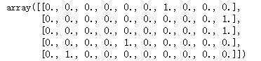
将标签改为独热编码

from sklearn.preprocessing import OneHotEncoder
encoder=OneHotEncoder(sparse=False)
yy=[[0],[1],[2],[3],[4],[5],[6],[7],[8],[9]]
encoder.fit(yy)
Ytrain_reshape=Ytrain.reshape(-1,1)
Ytrain_onehot=encoder.transform(Ytrain_reshape)
Ytest_reshape=Ytest.reshape(-1,1)
Ytest_onehot=encoder.transform(Ytest_reshape)

Ytrain_onehot.shape

Ytrain[:5]

Ytrain_onehot[:5]

5建立Cifar-10图像分类模型

具体模型如下

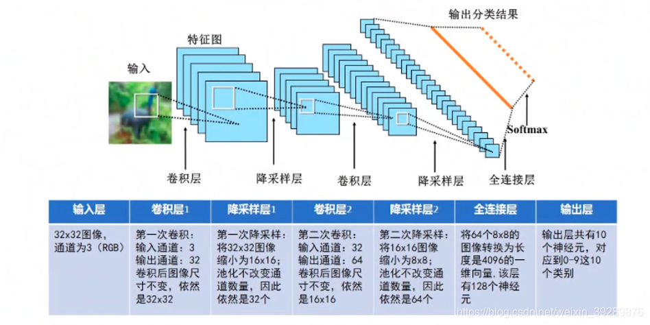
图像特征提取通过：卷积层1，降采样层1，卷积层2以及降采样层2处理提取图像特征
全连神经网络，全连接层，输出层所组成的网络结构

import tensorflow as tf
tf.reset_default_graph()

5.1定义共享函数

# 定义权值
def weight(shape):
    # 在构建模型时，需要使用tf.Variable来创建一个变量
    # 训练时变量不停更新
    #在使用函数tf.truncated_normal（截取正态分布）生成标准差为0.1的随机数来初始化权重
    return  tf.Variable(tf.truncated_normal(shape,stddev=0.1),name='W')
#定义偏置
#初始化0.1
def bias(shape):
    return tf.Variable(tf.constant(0.1,shape=shape),name='b')
#定义卷积操作
#步长为1.padding为‘SAME’
def conv2d(x,W):
    return tf.nn.conv2d(x,W,strides=[1,1,1,1],padding='SAME')
# 定义池化操作
# 步长为2，即原始长度长宽都除以2
def max_pool_22(x):
    return tf.nn.max_pool(x,ksize=[1,2,2,1],strides=[1,2,2,1],padding='SAME')

5.2定义网络结构

# 输入层
# 32*32图像通道为3（RGB）
with tf.name_scope('input_layer'):
    x=tf.placeholder('float',shape=[None,32,32,3],name='x')
# 第一个卷积层
# 输入通道为3，输出通道为32，卷积后图像尺寸不变，依然是32*32
with tf.name_scope('conv_1'):
    W1=weight([3,3,3,32])#1卷积核的宽，卷积核的高，输入通道，输出通道数量
    b1=bias([32])
    conv_1=conv2d(x,W1)+b1
    conv_1=tf.nn.relu(conv_1)
#第一个池化层
#将32*32图像缩小到16*16，池化不改变通道数量，因此还是32个
with tf.name_scope('pool_1'):
    pool_1=max_pool_22(conv_1)
#第二个卷积层
#输入通道：32.输出通道：64，卷积后尺寸不变，依然是16*16
with tf.name_scope('conv_2'):
    W2=weight([3,3,32,64])#1卷积核的宽，卷积核的高，输入通道，输出通道数量
    b2=bias([64])
    conv_2=conv2d(pool_1,W2)+b2
    conv_2=tf.nn.relu(conv_2)
#第2个池化层
#将16*16图像缩小到8*8，池化不改变通道数量，因此还是32个
with tf.name_scope('pool_2'):
    pool_2=max_pool_22(conv_2)
# 全连接层
# 将池化第二个池化层的64个8*8图像转为1维向量，长度是64*8*8=4096
with tf.name_scope('fc'):
    W3=weight([4096,128])
    b3=bias([128])
    flat=tf.reshape(pool_2,[-1,4096])
    h=tf.nn.relu(tf.matmul(flat,W3)+b3)
    h_dropout=tf.nn.dropout(h,keep_prob=0.8)#加入dropout避免过拟合
#再加入一层池化层
with tf.name_scope('fc2'):
    W4=weight([128,128])
    b4=bias([128])
    h2=tf.nn.relu(tf.matmul(h_dropout,W4)+b4)
    h_dropout2=tf.nn.dropout(h2,keep_prob=0.8)#加入dropout避免过拟合
#输出层
#输出层共有10个神经元，对应0-9个类别
with tf.name_scope('output_layer'):
    W5=weight([128,10])
    b5=bias([10])
    pred=tf.nn.softmax(tf.matmul(h_dropout,W5)+b5)

5.3构建模型

with tf.name_scope('optimizer'):
    # 定义占位符
    y=tf.placeholder('float',shape=[None,10],name='label')
    #定义损失函数
    loss_function=tf.reduce_mean(tf.nn.softmax_cross_entropy_with_logits(logits=pred,labels=y))
    #选择优化器
    optimizer=tf.train.AdamOptimizer(learning_rate=0.0001).minimize(loss_function)

5.4定义准确率

with tf.name_scope("evolution"):
    correct_prediction=tf.equal(tf.argmax(pred,1),tf.argmax(y,1))
    accuracy=tf.reduce_mean(tf.cast(correct_prediction,'float'))

6训练

6.1启动会话

import os 
from time import time
train_epochs=50
batch_size=50
total_batch=int(len(Xtrain)/batch_size)
epoch_list=[]
accuracy_list=[]
loss_list=[]
epoch=tf.Variable(0,name='epoch',trainable=False)
startTime=time()
sess=tf.Session()
init=tf.global_variables_initializer()
sess.run(init)

6.2断点续训

#  设置检查点存储目录
ckpt_dir='CIFAR10_log/'
if not os.path.exists(ckpt_dir):
    os.makedirs(ckpt_dir)
#生成saver
saver=tf.train.Saver(max_to_keep=1)
# 如果有检查点文件，读取最新检查文件，恢复各种变量值
ckpt=tf.train.latest_checkpoint(ckpt_dir)
if ckpt!= None:
    saver.restore(sess,ckpt)#加载所有参数
    #从这里接上次训练的轮数
else:
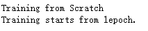
    print('Training from Scratch')
# 获取续训数据
start=sess.run(epoch)
print('Training starts from {}epoch.'.format(start+1))

6.3迭代训练

def get_train_batch(number,batch_size):
    return Xtrain_normalize[number*batch_size:(number+1)*batch_size],\
            Ytrain_onehot[number*batch_size:(number+1)*batch_size]
for ep in range(start,train_epochs):
    for i in range(total_batch):
        batch_x,batch_y=get_train_batch(i,batch_size)
        sess.run(optimizer,feed_dict={x:batch_x,y:batch_y})
        if i%100==0:
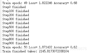
            print('Step{}'.format(i),'finished')
    
    loss,acc=sess.run([loss_function,accuracy],feed_dict={x:batch_x,y:batch_y})
    epoch_list.append(ep+1)
    loss_list.append(loss)
    accuracy_list.append(acc)
    print('Train epoch:','%02d'%(sess.run(epoch)+1),\
         'Loss=','{:.6f}'.format(loss),'Accuracy=',acc)
    #保存检查点
    saver.save(sess,ckpt_dir+'CIFAR10_cnn_model.ckpt',global_step=ep+1)
    sess.run(epoch.assign(ep+1))
duration=time()-startTime
print('Train finished takes:',duration

最后准确率在68左右

7模型预测

7.1计算测试集上准确率

test_total_batch=int(len(Xtest_normalize)/batch_size)
test_acc_sum=0.0
for i in range(test_total_batch):
    test_image_batch=Xtest_normalize[i*batch_size:(i+1)*batch_size]
    test_label_batch=Ytest_onehot[i*batch_size:(i+1)*batch_size]
    test_batch_acc=sess.run(accuracy,feed_dict={x:test_image_batch,y:test_label_batch})
    test_acc_sum+=test_batch_acc
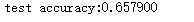
test_acc=float(test_acc_sum/test_total_batch)
print('test accuracy:{:.6f}'.format(test_acc))

7.2利用模型进行预测

test_pred=sess.run(pred,feed_dict={x:Xtest_normalize[:10]})
prediction_result=sess.run(tf.argmax(test_pred,1))

7.3 可视化预测结果

plot_images_labels_prediction(Xtest,Ytest,prediction_result,0,10)