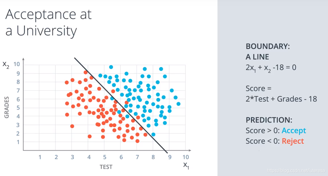
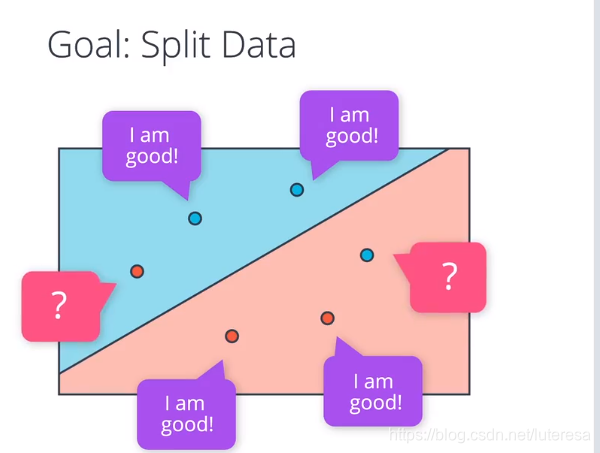
分类问题
在二维空间,实际上可以等效于拟合最佳直线,将所有点分类
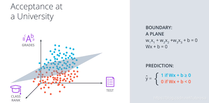
三围空间,就是拟合最佳平面
扩展到n维空间
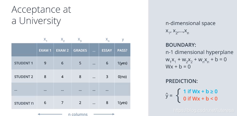
满足n维空间的各向量维度
W:(1xn), x:(nx1), b:(1x1)
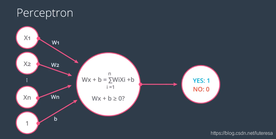
感知器
把方程式进行编码,形成下图的节点链接方式
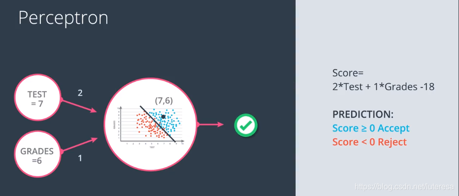
把方程式参数提取出来作为权重,特征向量作为输入节点,方程结果作为输出
把偏置值也作为一个权重(对应特征为固定值1),最后检查结果是否大于0,如果是,返回1,否则返回0;
提炼出通用公式:
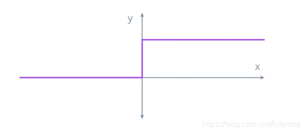
阶跃函数 Setp Function
输入值不小于0,则输出1,否则输出0;
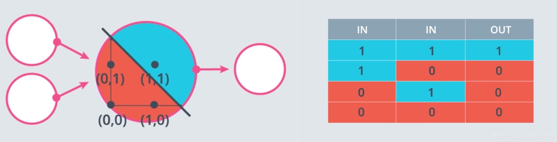
用感知器实现简单逻辑
AND运算
%matplotlib inline
import pandas as pd

# TODO: Set weight1, weight2, and bias
weight1 = 1.0
weight2 = 1.0
bias = -1.5


# DON'T CHANGE ANYTHING BELOW
# Inputs and outputs
test_inputs = [(0, 0), (0, 1), (1, 0), (1, 1)]
correct_outputs = [False, False, False, True]
outputs = []

# Generate and check output
for test_input, correct_output in zip(test_inputs, correct_outputs):
    linear_combination = weight1 * test_input[0] + weight2 * test_input[1] + bias
    output = int(linear_combination >= 0)
    is_correct_string = 'Yes' if output == correct_output else 'No'
    outputs.append([test_input[0], test_input[1], linear_combination, output, is_correct_string])

# Print output
num_wrong = len([output[4] for output in outputs if output[4] == 'No'])
output_frame = pd.DataFrame(outputs, columns=['Input 1', '  Input 2', '  Linear Combination', '  Activation Output', '  Is Correct'])
if not num_wrong:
    print('Nice!  You got it all correct.\n')
else:
    print('You got {} wrong.  Keep trying!\n'.format(num_wrong))
print(output_frame.to_string(index=False))
Nice!  You got it all correct.

 Input 1    Input 2    Linear Combination    Activation Output   Is Correct
       0          0                  -1.5                    0          Yes
       0          1                  -0.5                    0          Yes
       1          0                  -0.5                    0          Yes
       1          1                   0.5                    1          Yes
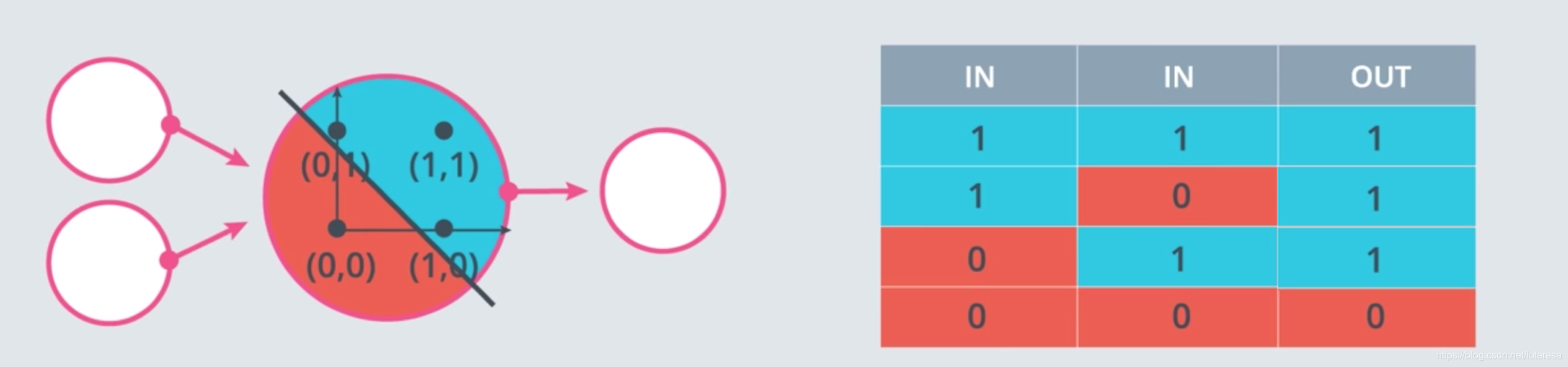
OR 运算
NOT (‘非’)
%matplotlib inline
import pandas as pd

# TODO: Set weight1, weight2, and bias
weight1 = 2.5
weight2 = -4.5
bias = 1.0


# DON'T CHANGE ANYTHING BELOW
# Inputs and outputs
test_inputs = [(0, 0), (0, 1), (1, 0), (1, 1)]
correct_outputs = [True, False, True, False]
outputs = []

# Generate and check output
for test_input, correct_output in zip(test_inputs, correct_outputs):
    linear_combination = weight1 * test_input[0] + weight2 * test_input[1] + bias
    output = int(linear_combination >= 0)
    is_correct_string = 'Yes' if output == correct_output else 'No'
    outputs.append([test_input[0], test_input[1], linear_combination, output, is_correct_string])

# Print output
num_wrong = len([output[4] for output in outputs if output[4] == 'No'])
output_frame = pd.DataFrame(outputs, columns=['Input 1', '  Input 2', '  Linear Combination', '  Activation Output', '  Is Correct'])
if not num_wrong:
    print('Nice!  You got it all correct.\n')
else:
    print('You got {} wrong.  Keep trying!\n'.format(num_wrong))
print(output_frame.to_string(index=False))
Nice!  You got it all correct.

 Input 1    Input 2    Linear Combination    Activation Output   Is Correct
       0          0                   1.0                    1          Yes
       0          1                  -3.5                    0          Yes
       1          0                   3.5                    1          Yes
       1          1                  -1.0                    0          Yes
用感知器实现逻辑运算 - XOR (“异或”)
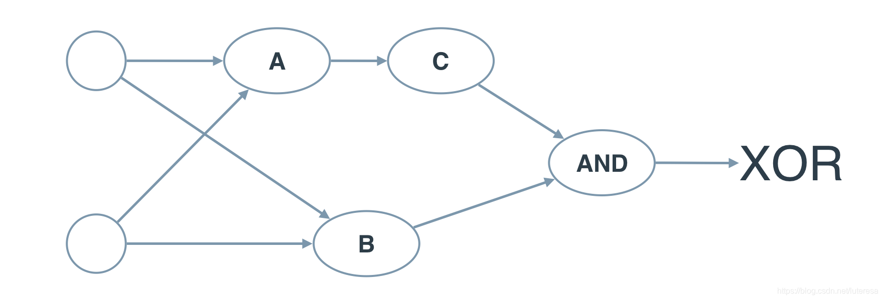
A: AND
B: OR
C: NOT
通过简单逻辑的重新组合,可以表达更复杂的逻辑。
感知器是神经网络的最基础单元,
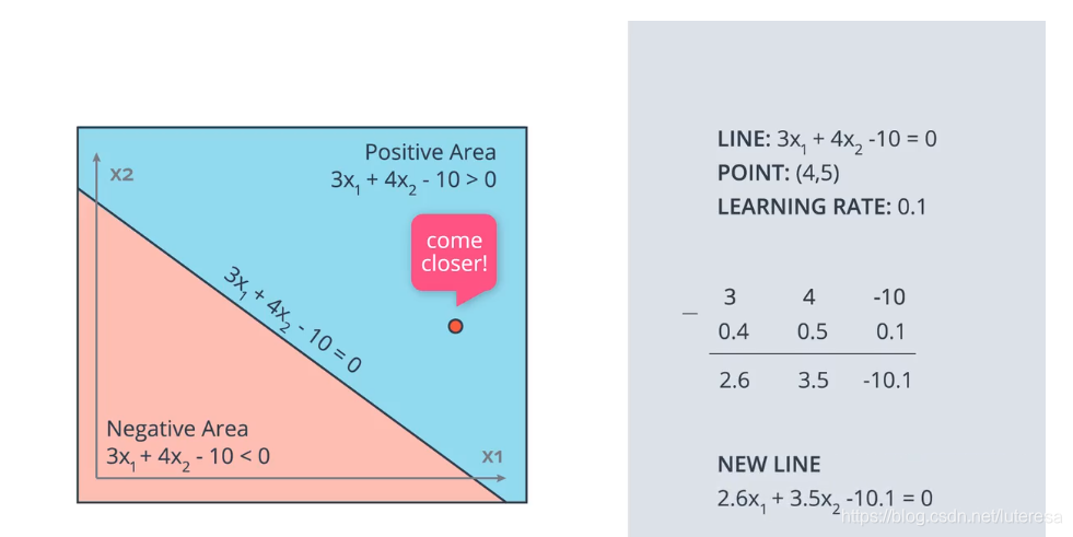
如何拟合最佳感知器方程?
先给待拟合参数任意初始值,然后检查所有学习数据
正确分类的点,不做处理,凡发现错误点,更新参数,使分类直线更靠近自己
调整直线,更新参数的方法,类似线性回归中的拟合直线
感知器算法实现
import numpy as np
# Setting the random seed, feel free to change it and see different solutions.
np.random.seed(42)
def stepFunction(t):
if t >= 0:
return 1
return 0
def prediction(X, W, b):
return stepFunction((np.matmul(X,W)+b)[0])
# TODO: Fill in the code below to implement the perceptron trick.
# The function should receive as inputs the data X, the labels y,
# the weights W (as an array), and the bias b,
# update the weights and bias W, b, according to the perceptron algorithm,
# and return W and b.
def perceptronStep(X, y, W, b, learn_rate = 0.01):
# Fill in code
for i in range(len(X)):
y_hat = prediction(X[i],W,b)
if y[i]-y_hat == 1:
W[0] += X[i][0]*learn_rate
W[1] += X[i][1]*learn_rate
b += learn_rate
elif y[i]-y_hat == -1:
W[0] -= X[i][0]*learn_rate
W[1] -= X[i][1]*learn_rate
b -= learn_rate
return W, b
# This function runs the perceptron algorithm repeatedly on the dataset,
# and returns a few of the boundary lines obtained in the iterations,
# for plotting purposes.
# Feel free to play with the learning rate and the num_epochs,
# and see your results plotted below.
def trainPerceptronAlgorithm(X, y, learn_rate = 0.01, num_epochs = 25):
x_min, x_max = min(X.T[0]), max(X.T[0])
y_min, y_max = min(X.T[1]), max(X.T[1])
W = np.array(np.random.rand(2,1))
b = np.random.rand(1)[0] + x_max
# These are the solution lines that get plotted below.
boundary_lines = []
for i in range(num_epochs):
# In each epoch, we apply the perceptron step.
W, b = perceptronStep(X, y, W, b, learn_rate)
boundary_lines.append((-W[0]/W[1], -b/W[1]))
return boundary_lines
if __name__ == "__main__":
# perform perceptron
data = np.loadtxt('data.csv', delimiter = ',')
print("data.type:",type(data),data.reshape)
X = data[:,:-1]
y = data[:,-1]
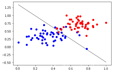
regression_coef = trainPerceptronAlgorithm(X, y) #返回训练过程多组系数
# plot the results
import matplotlib.pyplot as plt
plt.figure()
X_ = data[:,0]
y_ = data[:,1]
data1 = [x for x in data if x[2] > 0]
data0 = [x for x in data if x[2] == 0]
X_min = X_.min()
X_max = X_.max()
data0_ = np.array(data0)
X0_ = data0_[:,0]
Y0_ = data0_[:,1]
data1_ = np.array(data1)
X1_ = data1_[:,0]
Y1_ = data1_[:,1]
plt.scatter(X1_, Y1_, zorder = 3, c='b')
plt.scatter(X0_, Y0_, zorder = 3, c='r')
counter = len(regression_coef)
#print(regression_coef)
'''
想画多根直线,直观看分类线移动过程,代码有问题
for W, b in regression_coef:
counter -= 1
color = [1 - 0.92 ** counter for _ in range(3)]
#print(color)
Y_min = X_min * W + b
Y_max = X_max * W + b
if Y_min > 1:
Y_min = 1
X_min = (1 - b)/W
if Y_min < 0:
Y_min = 0
X_min = (0-b)/W
if Y_max > 1:
Y_max = 1
X_max = (1 - b)/W
if Y_max < 0:
Y_max = 0
X_max = (Y_max - b)/W
print([X_min, X_max],[Y_min, Y_max])
#plt.plot([X_min, X_max],[Y_min, Y_max], color = color) #color=[0.5, 0.5, 0.5]
'''
W, b = regression_coef[-1]
plt.plot([X_min, X_max],[X_min * W + b, X_max * W + b], color=[0.5, 0.5, 0.5])
#plt.show()
plt.savefig("Perceptron.png")
感知器是神经网络基础,类似人脑神经中的神经元,神经网络是由多个感知器,按不同规则组合成不同网络模型。
