分类问题

神经网络是机器学习中的一个模型，可以用于两类问题的解答：

分类：把数据划分成不同的类别
回归：建立数据间的连续关系

什么是分类问题？分类（classification），即找一个函数判断输入数据所属的类别，可以是二类别问题（是/不是），也可以是多类别问题（在多个类别中判断输入数据具体属于哪一个类别）。与回归问题（regression）相比，分类问题的输出不再是连续值，而是离散值，用来指定其属于哪个类别。分类问题在现实中应用非常广泛，比如垃圾邮件识别，手写数字识别，人脸识别，语音识别等。

线性界线

W为权重，b为偏差。

更高维度的界线

感知器

多层感知器的结构，称之为神经网络。

用感知器实现简单逻辑运算

实现AND（与）、OR（或）、NOT（非），XOR（异或）。

感知器技巧——计算机如何“学习”分类

这个分类方法，个人感觉像绝对值误差方法。整个数据集中的每一个点都会把分类的结果提供给感知器（分类函数），并调整感知器。——这就是计算机在神经网络算法中，找寻最优感知器的原理。

感知器算法

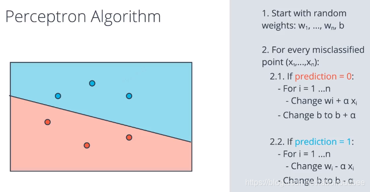
感知器步骤如下所示。对于坐标轴为 (p,q)(p,q) 的点，标签 y，以及等式 \hat{y} = step(w_1x_1 + w_2x_2 + b)y^=step(w1x1+w2x2+b) 给出的预测

如果点分类正确，则什么也不做。
如果点分类为正，但是标签为负，则分别减去 \alpha p, \alpha q,αp,αq, 和 \alphaα 至 w_1, w_2,w1,w2, 和 bb
如果点分类为负，但是标签为正，则分别将 \alpha p, \alpha q,αp,αq, 和 \alphaα 加到 w_1, w_2,w1,w2, 和 bb 上。

import numpy as np
# Setting the random seed, feel free to change it and see different solutions.
np.random.seed(42)

def stepFunction(t):
    if t >= 0:
        return 1
    return 0

def prediction(X, W, b):
    return stepFunction((np.matmul(X,W)+b)[0])

# TODO: Fill in the code below to implement the perceptron trick.
# The function should receive as inputs the data X, the labels y,
# the weights W (as an array), and the bias b,
# update the weights and bias W, b, according to the perceptron algorithm,
# and return W and b.
def perceptronStep(X, y, W, b, learn_rate = 0.01):
    # Fill in code
    for i in range(len(X)):
        y_hat = prediction(X[i], W, b)
        if y[i] - y_hat == 1:   #分类为负，标签为正
            W[0] += X[i][0] * learn_rate
            W[1] += X[i][1] * learn_rate
            b += learn_rate
        if y[i] - y_hat == -1:
            W[0] -= X[i][0] * learn_rate
            W[1] -= X[i][1] * learn_rate
            b -= learn_rate
    return W, b
    
# This function runs the perceptron algorithm repeatedly on the dataset,
# and returns a few of the boundary lines obtained in the iterations,
# for plotting purposes.
# Feel free to play with the learning rate and the num_epochs,
# and see your results plotted below.
def trainPerceptronAlgorithm(X, y, learn_rate = 0.01, num_epochs = 25):
    x_min, x_max = min(X.T[0]), max(X.T[0])
    y_min, y_max = min(X.T[1]), max(X.T[1])
    W = np.array(np.random.rand(2,1))
    b = np.random.rand(1)[0] + x_max
    # These are the solution lines that get plotted below.
    boundary_lines = []
    for i in range(num_epochs):
        # In each epoch, we apply the perceptron step.
        W, b = perceptronStep(X, y, W, b, learn_rate)
        boundary_lines.append((-W[0]/W[1], -b/W[1]))
    return boundary_lines

监督学习——感知器算法