Datawhale打卡第2次

EDA (Exploratory Data Analysis)，也就是对数据进行探索性的分析，从而为之后的数据预处理和特征工程提供必要的结论。
通常我们用到pandas库和可视化工具如 matplotlib 和 seaborn 就可以完成了。主要的步骤是：理解问题；读取数据；单变量探索；多变量探索；数据预处理；建立假设，并检验。
本次对二手车价格数据EDA的整个过程我用代码记录了下来，下面是我代码的一些展示，不再用过多的语言描述。

import warnings
warnings.filterwarnings('ignore')
import pandas as pd
import numpy as np
import matplotlib.pyplot as plt
import seaborn as sns
import missingno as msno
%matplotlib inline

Train_data = pd.read_csv('used_car_train_20200313.csv', sep=' ')#导入训练集
Test_data = pd.read_csv('used_car_testA_20200313.csv', sep=' ')#导入测试集

Train_data.head().append(Train_data.tail())#简单查看数据

	SaleID	name	regDate	model	brand	bodyType	fuelType	gearbox	power	kilometer	...	v_5	v_6	v_7	v_8	v_9	v_10	v_11	v_12	v_13	v_14
0	0	736	20040402	30.0	6	1.0	0.0	0.0	60	12.5	...	0.235676	0.101988	0.129549	0.022816	0.097462	-2.881803	2.804097	-2.420821	0.795292	0.914762
1	1	2262	20030301	40.0	1	2.0	0.0	0.0	0	15.0	...	0.264777	0.121004	0.135731	0.026597	0.020582	-4.900482	2.096338	-1.030483	-1.722674	0.245522
2	2	14874	20040403	115.0	15	1.0	0.0	0.0	163	12.5	...	0.251410	0.114912	0.165147	0.062173	0.027075	-4.846749	1.803559	1.565330	-0.832687	-0.229963
3	3	71865	19960908	109.0	10	0.0	0.0	1.0	193	15.0	...	0.274293	0.110300	0.121964	0.033395	0.000000	-4.509599	1.285940	-0.501868	-2.438353	-0.478699
4	4	111080	20120103	110.0	5	1.0	0.0	0.0	68	5.0	...	0.228036	0.073205	0.091880	0.078819	0.121534	-1.896240	0.910783	0.931110	2.834518	1.923482
149995	149995	163978	20000607	121.0	10	4.0	0.0	1.0	163	15.0	...	0.280264	0.000310	0.048441	0.071158	0.019174	1.988114	-2.983973	0.589167	-1.304370	-0.302592
149996	149996	184535	20091102	116.0	11	0.0	0.0	0.0	125	10.0	...	0.253217	0.000777	0.084079	0.099681	0.079371	1.839166	-2.774615	2.553994	0.924196	-0.272160
149997	149997	147587	20101003	60.0	11	1.0	1.0	0.0	90	6.0	...	0.233353	0.000705	0.118872	0.100118	0.097914	2.439812	-1.630677	2.290197	1.891922	0.414931
149998	149998	45907	20060312	34.0	10	3.0	1.0	0.0	156	15.0	...	0.256369	0.000252	0.081479	0.083558	0.081498	2.075380	-2.633719	1.414937	0.431981	-1.659014
149999	149999	177672	19990204	19.0	28	6.0	0.0	1.0	193	12.5	...	0.284475	0.000000	0.040072	0.062543	0.025819	1.978453	-3.179913	0.031724	-1.483350	-0.342674

10 rows × 31 columns

Train_data.shape

(150000, 31)

Test_data.head().append(Test_data.tail())#简单查看测试集

	SaleID	name	regDate	model	brand	bodyType	fuelType	gearbox	power	kilometer	...	v_5	v_6	v_7	v_8	v_9	v_10	v_11	v_12	v_13	v_14
0	150000	66932	20111212	222.0	4	5.0	1.0	1.0	313	15.0	...	0.264405	0.121800	0.070899	0.106558	0.078867	-7.050969	-0.854626	4.800151	0.620011	-3.664654
1	150001	174960	19990211	19.0	21	0.0	0.0	0.0	75	12.5	...	0.261745	0.000000	0.096733	0.013705	0.052383	3.679418	-0.729039	-3.796107	-1.541230	-0.757055
2	150002	5356	20090304	82.0	21	0.0	0.0	0.0	109	7.0	...	0.260216	0.112081	0.078082	0.062078	0.050540	-4.926690	1.001106	0.826562	0.138226	0.754033
3	150003	50688	20100405	0.0	0	0.0	0.0	1.0	160	7.0	...	0.260466	0.106727	0.081146	0.075971	0.048268	-4.864637	0.505493	1.870379	0.366038	1.312775
4	150004	161428	19970703	26.0	14	2.0	0.0	0.0	75	15.0	...	0.250999	0.000000	0.077806	0.028600	0.081709	3.616475	-0.673236	-3.197685	-0.025678	-0.101290
49995	199995	20903	19960503	4.0	4	4.0	0.0	0.0	116	15.0	...	0.284664	0.130044	0.049833	0.028807	0.004616	-5.978511	1.303174	-1.207191	-1.981240	-0.357695
49996	199996	708	19991011	0.0	0	0.0	0.0	0.0	75	15.0	...	0.268101	0.108095	0.066039	0.025468	0.025971	-3.913825	1.759524	-2.075658	-1.154847	0.169073
49997	199997	6693	20040412	49.0	1	0.0	1.0	1.0	224	15.0	...	0.269432	0.105724	0.117652	0.057479	0.015669	-4.639065	0.654713	1.137756	-1.390531	0.254420
49998	199998	96900	20020008	27.0	1	0.0	0.0	1.0	334	15.0	...	0.261152	0.000490	0.137366	0.086216	0.051383	1.833504	-2.828687	2.465630	-0.911682	-2.057353
49999	199999	193384	20041109	166.0	6	1.0	NaN	1.0	68	9.0	...	0.228730	0.000300	0.103534	0.080625	0.124264	2.914571	-1.135270	0.547628	2.094057	-1.552150

10 rows × 30 columns

Test_data.shape

(50000, 30)

Train_data.columns

Index(['SaleID', 'name', 'regDate', 'model', 'brand', 'bodyType', 'fuelType',
       'gearbox', 'power', 'kilometer', 'notRepairedDamage', 'regionCode',
       'seller', 'offerType', 'creatDate', 'price', 'v_0', 'v_1', 'v_2', 'v_3',
       'v_4', 'v_5', 'v_6', 'v_7', 'v_8', 'v_9', 'v_10', 'v_11', 'v_12',
       'v_13', 'v_14'],
      dtype='object')

Test_data.columns

Index(['SaleID', 'name', 'regDate', 'model', 'brand', 'bodyType', 'fuelType',
       'gearbox', 'power', 'kilometer', 'notRepairedDamage', 'regionCode',
       'seller', 'offerType', 'creatDate', 'v_0', 'v_1', 'v_2', 'v_3', 'v_4',
       'v_5', 'v_6', 'v_7', 'v_8', 'v_9', 'v_10', 'v_11', 'v_12', 'v_13',
       'v_14'],
      dtype='object')

Train_data.describe()#熟悉数据的相关统计量

	SaleID	name	regDate	model	brand	bodyType	fuelType	gearbox	power	kilometer	...	v_5	v_6	v_7	v_8	v_9	v_10	v_11	v_12	v_13	v_14
count	150000.000000	150000.000000	1.500000e+05	149999.000000	150000.000000	145494.000000	141320.000000	144019.000000	150000.000000	150000.000000	...	150000.000000	150000.000000	150000.000000	150000.000000	150000.000000	150000.000000	150000.000000	150000.000000	150000.000000	150000.000000
mean	74999.500000	68349.172873	2.003417e+07	47.129021	8.052733	1.792369	0.375842	0.224943	119.316547	12.597160	...	0.248204	0.044923	0.124692	0.058144	0.061996	-0.001000	0.009035	0.004813	0.000313	-0.000688
std	43301.414527	61103.875095	5.364988e+04	49.536040	7.864956	1.760640	0.548677	0.417546	177.168419	3.919576	...	0.045804	0.051743	0.201410	0.029186	0.035692	3.772386	3.286071	2.517478	1.288988	1.038685
min	0.000000	0.000000	1.991000e+07	0.000000	0.000000	0.000000	0.000000	0.000000	0.000000	0.500000	...	0.000000	0.000000	0.000000	0.000000	0.000000	-9.168192	-5.558207	-9.639552	-4.153899	-6.546556
25%	37499.750000	11156.000000	1.999091e+07	10.000000	1.000000	0.000000	0.000000	0.000000	75.000000	12.500000	...	0.243615	0.000038	0.062474	0.035334	0.033930	-3.722303	-1.951543	-1.871846	-1.057789	-0.437034
50%	74999.500000	51638.000000	2.003091e+07	30.000000	6.000000	1.000000	0.000000	0.000000	110.000000	15.000000	...	0.257798	0.000812	0.095866	0.057014	0.058484	1.624076	-0.358053	-0.130753	-0.036245	0.141246
75%	112499.250000	118841.250000	2.007111e+07	66.000000	13.000000	3.000000	1.000000	0.000000	150.000000	15.000000	...	0.265297	0.102009	0.125243	0.079382	0.087491	2.844357	1.255022	1.776933	0.942813	0.680378
max	149999.000000	196812.000000	2.015121e+07	247.000000	39.000000	7.000000	6.000000	1.000000	19312.000000	15.000000	...	0.291838	0.151420	1.404936	0.160791	0.222787	12.357011	18.819042	13.847792	11.147669	8.658418

8 rows × 30 columns

Test_data.describe()

	SaleID	name	regDate	model	brand	bodyType	fuelType	gearbox	power	kilometer	...	v_5	v_6	v_7	v_8	v_9	v_10	v_11	v_12	v_13	v_14
count	50000.000000	50000.000000	5.000000e+04	50000.000000	50000.000000	48587.000000	47107.000000	48090.000000	50000.000000	50000.000000	...	50000.000000	50000.000000	50000.000000	50000.000000	50000.000000	50000.000000	50000.000000	50000.000000	50000.000000	50000.000000
mean	174999.500000	68542.223280	2.003393e+07	46.844520	8.056240	1.782185	0.373405	0.224350	119.883620	12.595580	...	0.248669	0.045021	0.122744	0.057997	0.062000	-0.017855	-0.013742	-0.013554	-0.003147	0.001516
std	14433.901067	61052.808133	5.368870e+04	49.469548	7.819477	1.760736	0.546442	0.417158	185.097387	3.908979	...	0.044601	0.051766	0.195972	0.029211	0.035653	3.747985	3.231258	2.515962	1.286597	1.027360
min	150000.000000	0.000000	1.991000e+07	0.000000	0.000000	0.000000	0.000000	0.000000	0.000000	0.500000	...	0.000000	0.000000	0.000000	0.000000	0.000000	-9.160049	-5.411964	-8.916949	-4.123333	-6.112667
25%	162499.750000	11203.500000	1.999091e+07	10.000000	1.000000	0.000000	0.000000	0.000000	75.000000	12.500000	...	0.243762	0.000044	0.062644	0.035084	0.033714	-3.700121	-1.971325	-1.876703	-1.060428	-0.437920
50%	174999.500000	52248.500000	2.003091e+07	29.000000	6.000000	1.000000	0.000000	0.000000	109.000000	15.000000	...	0.257877	0.000815	0.095828	0.057084	0.058764	1.613212	-0.355843	-0.142779	-0.035956	0.138799
75%	187499.250000	118856.500000	2.007110e+07	65.000000	13.000000	3.000000	1.000000	0.000000	150.000000	15.000000	...	0.265328	0.102025	0.125438	0.079077	0.087489	2.832708	1.262914	1.764335	0.941469	0.681163
max	199999.000000	196805.000000	2.015121e+07	246.000000	39.000000	7.000000	6.000000	1.000000	20000.000000	15.000000	...	0.291618	0.153265	1.358813	0.156355	0.214775	12.338872	18.856218	12.950498	5.913273	2.624622

8 rows × 29 columns

Train_data.info()#熟悉数据类型

<class 'pandas.core.frame.DataFrame'>
RangeIndex: 150000 entries, 0 to 149999
Data columns (total 31 columns):
SaleID               150000 non-null int64
name                 150000 non-null int64
regDate              150000 non-null int64
model                149999 non-null float64
brand                150000 non-null int64
bodyType             145494 non-null float64
fuelType             141320 non-null float64
gearbox              144019 non-null float64
power                150000 non-null int64
kilometer            150000 non-null float64
notRepairedDamage    150000 non-null object
regionCode           150000 non-null int64
seller               150000 non-null int64
offerType            150000 non-null int64
creatDate            150000 non-null int64
price                150000 non-null int64
v_0                  150000 non-null float64
v_1                  150000 non-null float64
v_2                  150000 non-null float64
v_3                  150000 non-null float64
v_4                  150000 non-null float64
v_5                  150000 non-null float64
v_6                  150000 non-null float64
v_7                  150000 non-null float64
v_8                  150000 non-null float64
v_9                  150000 non-null float64
v_10                 150000 non-null float64
v_11                 150000 non-null float64
v_12                 150000 non-null float64
v_13                 150000 non-null float64
v_14                 150000 non-null float64
dtypes: float64(20), int64(10), object(1)
memory usage: 35.5+ MB

Test_data.info()

<class 'pandas.core.frame.DataFrame'>
RangeIndex: 50000 entries, 0 to 49999
Data columns (total 30 columns):
SaleID               50000 non-null int64
name                 50000 non-null int64
regDate              50000 non-null int64
model                50000 non-null float64
brand                50000 non-null int64
bodyType             48587 non-null float64
fuelType             47107 non-null float64
gearbox              48090 non-null float64
power                50000 non-null int64
kilometer            50000 non-null float64
notRepairedDamage    50000 non-null object
regionCode           50000 non-null int64
seller               50000 non-null int64
offerType            50000 non-null int64
creatDate            50000 non-null int64
v_0                  50000 non-null float64
v_1                  50000 non-null float64
v_2                  50000 non-null float64
v_3                  50000 non-null float64
v_4                  50000 non-null float64
v_5                  50000 non-null float64
v_6                  50000 non-null float64
v_7                  50000 non-null float64
v_8                  50000 non-null float64
v_9                  50000 non-null float64
v_10                 50000 non-null float64
v_11                 50000 non-null float64
v_12                 50000 non-null float64
v_13                 50000 non-null float64
v_14                 50000 non-null float64
dtypes: float64(20), int64(9), object(1)
memory usage: 11.4+ MB

Train_data.isnull().sum()#查看缺失值情况

SaleID                  0
name                    0
regDate                 0
model                   1
brand                   0
bodyType             4506
fuelType             8680
gearbox              5981
power                   0
kilometer               0
notRepairedDamage       0
regionCode              0
seller                  0
offerType               0
creatDate               0
price                   0
v_0                     0
v_1                     0
v_2                     0
v_3                     0
v_4                     0
v_5                     0
v_6                     0
v_7                     0
v_8                     0
v_9                     0
v_10                    0
v_11                    0
v_12                    0
v_13                    0
v_14                    0
dtype: int64

Test_data.isnull().sum()

SaleID                  0
name                    0
regDate                 0
model                   0
brand                   0
bodyType             1413
fuelType             2893
gearbox              1910
power                   0
kilometer               0
notRepairedDamage       0
regionCode              0
seller                  0
offerType               0
creatDate               0
v_0                     0
v_1                     0
v_2                     0
v_3                     0
v_4                     0
v_5                     0
v_6                     0
v_7                     0
v_8                     0
v_9                     0
v_10                    0
v_11                    0
v_12                    0
v_13                    0
v_14                    0
dtype: int64

miss=Train_data.isnull().sum()
miss=miss[miss>0].sort_values()
miss.plot.bar()

<matplotlib.axes._subplots.AxesSubplot at 0x1e1f75f3518>

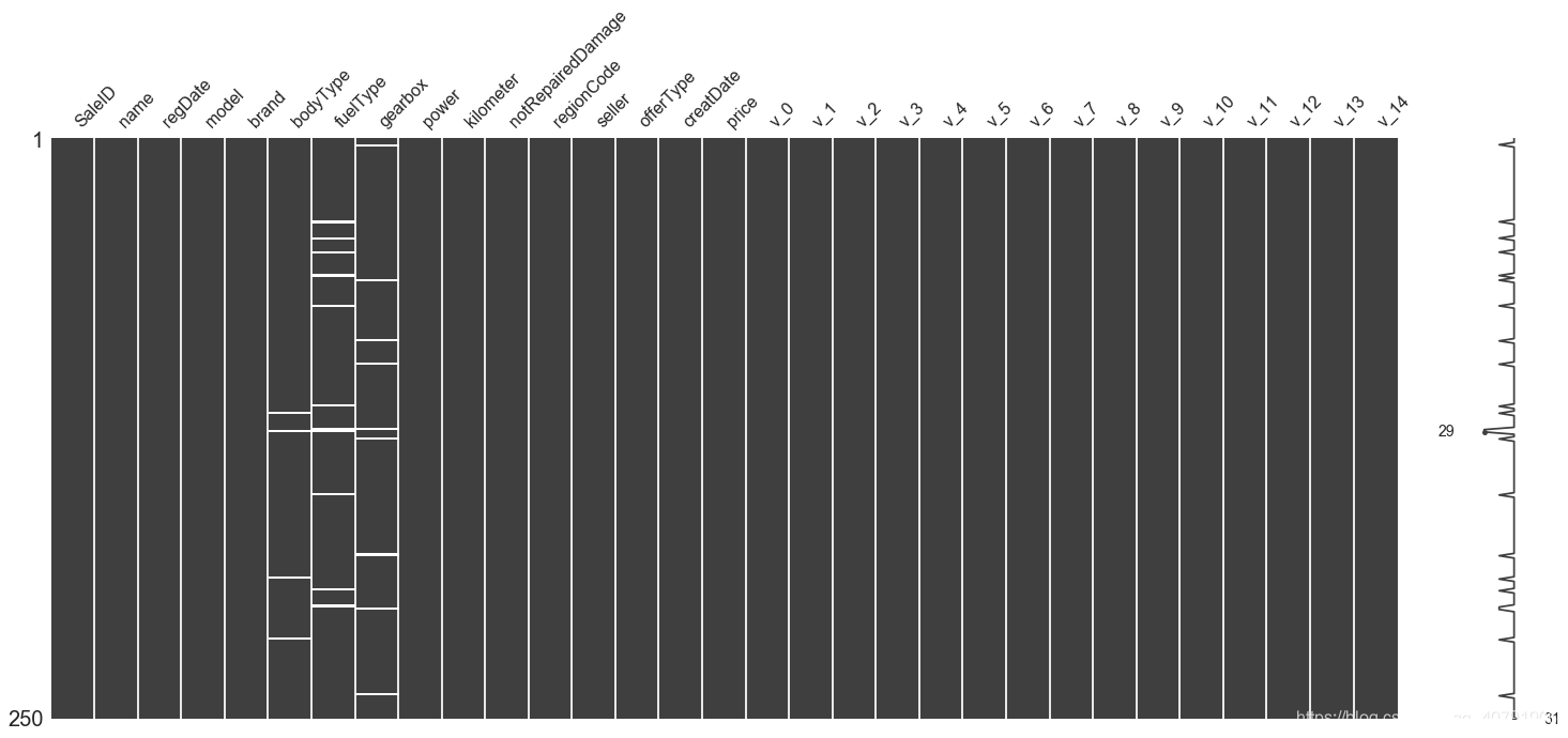
msno.matrix(Train_data.sample(250))#可视化看一下缺失值

<matplotlib.axes._subplots.AxesSubplot at 0x1e1f7558c50>

在这里插入图片描述

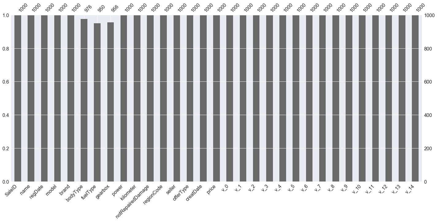
msno.bar(Train_data.sample(1000))

<matplotlib.axes._subplots.AxesSubplot at 0x1e1f903df60>

在这里插入图片描述

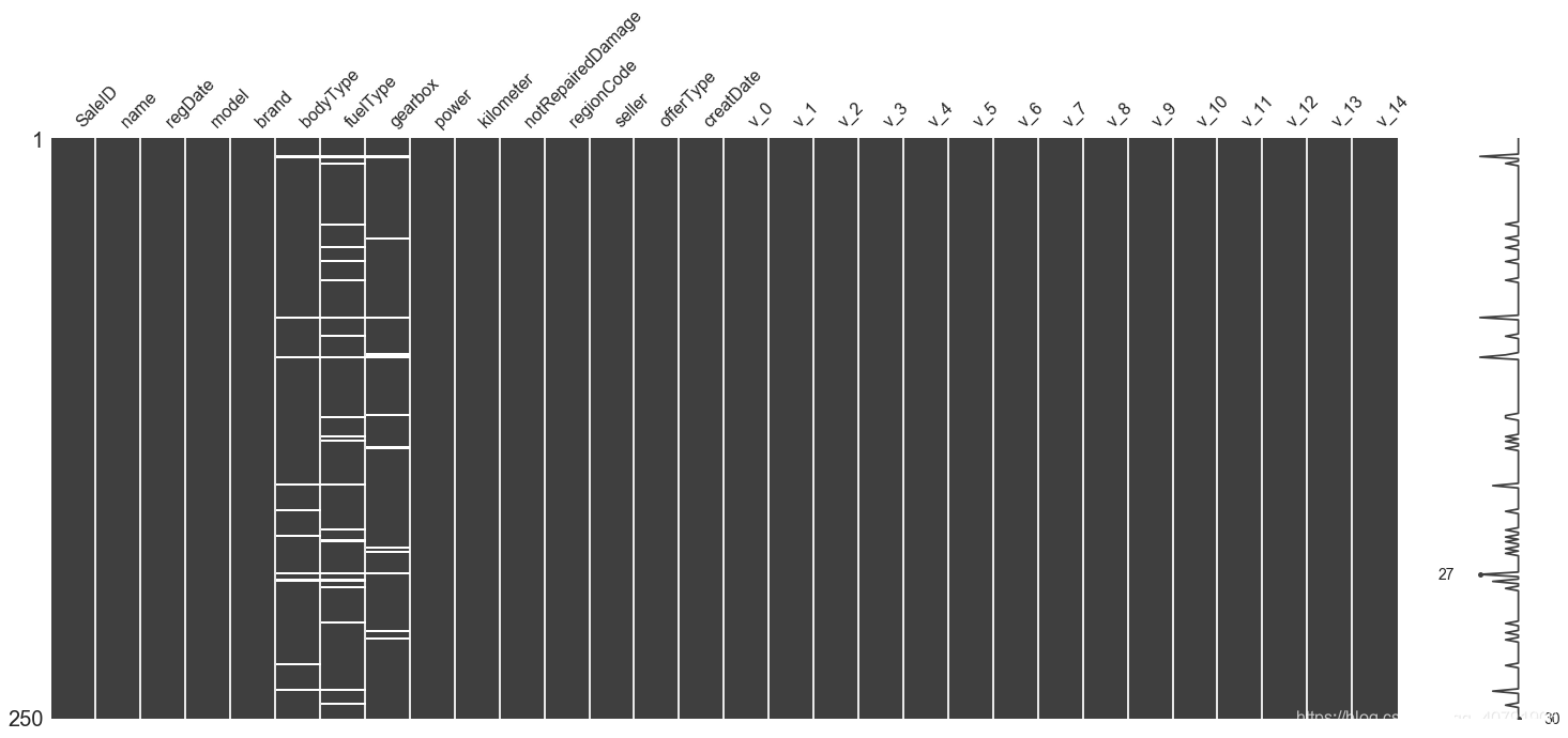
msno.matrix(Test_data.sample(250))

<matplotlib.axes._subplots.AxesSubplot at 0x1e1f9372be0>

在这里插入图片描述

msno.bar(Test_data.sample(1000))

<matplotlib.axes._subplots.AxesSubplot at 0x1e1f9330f60>

在这里插入图片描述

Train_data.info()

<class 'pandas.core.frame.DataFrame'>
RangeIndex: 150000 entries, 0 to 149999
Data columns (total 31 columns):
SaleID               150000 non-null int64
name                 150000 non-null int64
regDate              150000 non-null int64
model                149999 non-null float64
brand                150000 non-null int64
bodyType             145494 non-null float64
fuelType             141320 non-null float64
gearbox              144019 non-null float64
power                150000 non-null int64
kilometer            150000 non-null float64
notRepairedDamage    150000 non-null object
regionCode           150000 non-null int64
seller               150000 non-null int64
offerType            150000 non-null int64
creatDate            150000 non-null int64
price                150000 non-null int64
v_0                  150000 non-null float64
v_1                  150000 non-null float64
v_2                  150000 non-null float64
v_3                  150000 non-null float64
v_4                  150000 non-null float64
v_5                  150000 non-null float64
v_6                  150000 non-null float64
v_7                  150000 non-null float64
v_8                  150000 non-null float64
v_9                  150000 non-null float64
v_10                 150000 non-null float64
v_11                 150000 non-null float64
v_12                 150000 non-null float64
v_13                 150000 non-null float64
v_14                 150000 non-null float64
dtypes: float64(20), int64(10), object(1)
memory usage: 35.5+ MB

Train_data['notRepairedDamage'].value_counts()

0.0    111361
-       24324
1.0     14315
Name: notRepairedDamage, dtype: int64

Train_data['notRepairedDamage'].replace('-',np.nan,inplace=True)#将-替换为缺省值

Train_data['notRepairedDamage'].value_counts()

0.0    111361
1.0     14315
Name: notRepairedDamage, dtype: int64

Train_data.isnull().sum()#重新看一下缺省值多少

SaleID                   0
name                     0
regDate                  0
model                    1
brand                    0
bodyType              4506
fuelType              8680
gearbox               5981
power                    0
kilometer                0
notRepairedDamage    24324
regionCode               0
seller                   0
offerType                0
creatDate                0
price                    0
v_0                      0
v_1                      0
v_2                      0
v_3                      0
v_4                      0
v_5                      0
v_6                      0
v_7                      0
v_8                      0
v_9                      0
v_10                     0
v_11                     0
v_12                     0
v_13                     0
v_14                     0
dtype: int64

Test_data['notRepairedDamage'].replace('-',np.nan,inplace=True)

Test_data['notRepairedDamage'].value_counts()

0.0    37249
1.0     4720
Name: notRepairedDamage, dtype: int64

Train_data['seller'].value_counts()#此项可删掉

0    149999
1         1
Name: seller, dtype: int64

Train_data['offerType'].value_counts()#此项可删掉

0    150000
Name: offerType, dtype: int64

del Train_data["seller"]
del Train_data["offerType"]
del Test_data["seller"]
del Test_data["offerType"]

Train_data['price']#了解结果分布情况

0          1850
1          3600
2          6222
3          2400
4          5200
5          8000
6          3500
7          1000
8          2850
9           650
10         3100
11         5450
12         1600
13         3100
14         6900
15         3200
16        10500
17         3700
18          790
19         1450
20          990
21         2800
22          350
23          599
24         9250
25         3650
26         2800
27         2399
28         4900
29         2999
          ...  
149970      900
149971     3400
149972      999
149973     3500
149974     4500
149975     3990
149976     1200
149977      330
149978     3350
149979     5000
149980     4350
149981     9000
149982     2000
149983    12000
149984     6700
149985     4200
149986     2800
149987     3000
149988     7500
149989     1150
149990      450
149991    24950
149992      950
149993     4399
149994    14780
149995     5900
149996     9500
149997     7500
149998     4999
149999     4700
Name: price, Length: 150000, dtype: int64

Train_data['price'].value_counts()

500      2337
1500     2158
1200     1922
1000     1850
2500     1821
600      1535
3500     1533
800      1513
2000     1378
999      1356
750      1279
4500     1271
650      1257
1800     1223
2200     1201
850      1198
700      1174
900      1107
1300     1105
950      1104
3000     1098
1100     1079
5500     1079
1600     1074
300      1071
550      1042
350      1005
1250     1003
6500      973
1999      929
         ... 
21560       1
7859        1
3120        1
2279        1
6066        1
6322        1
4275        1
10420       1
43300       1
305         1
1765        1
15970       1
44400       1
8885        1
2992        1
31850       1
15413       1
13495       1
9525        1
7270        1
13879       1
3760        1
24250       1
11360       1
10295       1
25321       1
8886        1
8801        1
37920       1
8188        1
Name: price, Length: 3763, dtype: int64

import scipy.stats as st
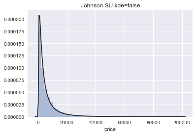
y = Train_data['price']
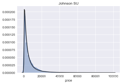
plt.figure(1); plt.title('Johnson SU')
sns.distplot(y, fit=st.johnsonsu)
plt.figure(2); plt.title('Johnson SU kde=false')
sns.distplot(y,kde=False, fit=st.johnsonsu)
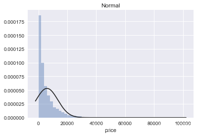
plt.figure(3); plt.title('Normal')
sns.distplot(y, kde=False, fit=st.norm)
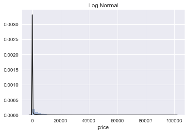
plt.figure(4); plt.title('Log Normal')
sns.distplot(y, kde=False, fit=st.lognorm)#查看价格的概率分布情况

<matplotlib.axes._subplots.AxesSubplot at 0x1e1fab9ddd8>

在这里插入图片描述

plt.figure(1); plt.title('Johnson SU hist=false')
sns.distplot(y,kde=False,hist=False, fit=st.johnsonsu)

<matplotlib.axes._subplots.AxesSubplot at 0x1e1f9a529b0>

在这里插入图片描述

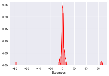
Train_data.skew(), Train_data.kurt()#看一下偏度和峰度

(SaleID               6.017846e-17
 name                 5.576058e-01
 regDate              2.849508e-02
 model                1.484388e+00
 brand                1.150760e+00
 bodyType             9.915299e-01
 fuelType             1.595486e+00
 gearbox              1.317514e+00
 power                6.586318e+01
 kilometer           -1.525921e+00
 notRepairedDamage    2.430640e+00
 regionCode           6.888812e-01
 creatDate           -7.901331e+01
 price                3.346487e+00
 v_0                 -1.316712e+00
 v_1                  3.594543e-01
 v_2                  4.842556e+00
 v_3                  1.062920e-01
 v_4                  3.679890e-01
 v_5                 -4.737094e+00
 v_6                  3.680730e-01
 v_7                  5.130233e+00
 v_8                  2.046133e-01
 v_9                  4.195007e-01
 v_10                 2.522046e-02
 v_11                 3.029146e+00
 v_12                 3.653576e-01
 v_13                 2.679152e-01
 v_14                -1.186355e+00
 dtype: float64, SaleID                 -1.200000
 name                   -1.039945
 regDate                -0.697308
 model                   1.740483
 brand                   1.076201
 bodyType                0.206937
 fuelType                5.880049
 gearbox                -0.264161
 power                5733.451054
 kilometer               1.141934
 notRepairedDamage       3.908072
 regionCode             -0.340832
 creatDate            6881.080328
 price                  18.995183
 v_0                     3.993841
 v_1                    -1.753017
 v_2                    23.860591
 v_3                    -0.418006
 v_4                    -0.197295
 v_5                    22.934081
 v_6                    -1.742567
 v_7                    25.845489
 v_8                    -0.636225
 v_9                    -0.321491
 v_10                   -0.577935
 v_11                   12.568731
 v_12                    0.268937
 v_13                   -0.438274
 v_14                    2.393526
 dtype: float64)

sns.distplot(Train_data.skew(),color='red',axlabel ='Skewness')

<matplotlib.axes._subplots.AxesSubplot at 0x1e1fafdbc88>

在这里插入图片描述

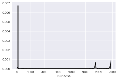
sns.distplot(Train_data.kurt(),color='black',axlabel ='Kurtness')

<matplotlib.axes._subplots.AxesSubplot at 0x1e1822d33c8>

在这里插入图片描述

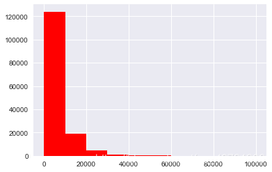
plt.hist(Train_data['price'], orientation = 'vertical',histtype = 'bar', color ='red')
plt.show()#查看价格数量

在这里插入图片描述

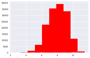
plt.hist(np.log(Train_data['price']), orientation = 'vertical',histtype = 'bar', color ='red') 
plt.show()

在这里插入图片描述

# 分离label即预测值
Y_train = Train_data['price']

numeric_features = ['power', 'kilometer', 'v_0', 'v_1', 'v_2', 'v_3', 'v_4', 'v_5', 'v_6', 'v_7', 'v_8', 'v_9', 'v_10', 'v_11', 'v_12', 'v_13','v_14' ]

categorical_features = ['name', 'model', 'brand', 'bodyType', 'fuelType', 'gearbox', 'notRepairedDamage', 'regionCode',]

# 特征nunique分布
for cat_fea in categorical_features:
    print(cat_fea + "的特征分布如下：")
    print("{}特征有个{}不同的值".format(cat_fea, Train_data[cat_fea].nunique()))
    print(Train_data[cat_fea].value_counts())

name的特征分布如下：
name特征有个99662不同的值
708       282
387       282
55        280
1541      263
203       233
53        221
713       217
290       197
1186      184
911       182
2044      176
1513      160
1180      158
631       157
893       153
2765      147
473       141
1139      137
1108      132
444       129
306       127
2866      123
2402      116
533       114
1479      113
422       113
4635      110
725       110
964       109
1373      104
         ... 
89083       1
95230       1
164864      1
173060      1
179207      1
181256      1
185354      1
25564       1
19417       1
189324      1
162719      1
191373      1
193422      1
136082      1
140180      1
144278      1
146327      1
148376      1
158621      1
1404        1
15319       1
46022       1
64463       1
976         1
3025        1
5074        1
7123        1
11221       1
13270       1
174485      1
Name: name, Length: 99662, dtype: int64
model的特征分布如下：
model特征有个248不同的值
0.0      11762
19.0      9573
4.0       8445
1.0       6038
29.0      5186
48.0      5052
40.0      4502
26.0      4496
8.0       4391
31.0      3827
13.0      3762
17.0      3121
65.0      2730
49.0      2608
46.0      2454
30.0      2342
44.0      2195
5.0       2063
10.0      2004
21.0      1872
73.0      1789
11.0      1775
23.0      1696
22.0      1524
69.0      1522
63.0      1469
7.0       1460
16.0      1349
88.0      1309
66.0      1250
         ...  
141.0       37
133.0       35
216.0       30
202.0       28
151.0       26
226.0       26
231.0       23
234.0       23
233.0       20
198.0       18
224.0       18
227.0       17
237.0       17
220.0       16
230.0       16
239.0       14
223.0       13
236.0       11
241.0       10
232.0       10
229.0       10
235.0        7
246.0        7
243.0        4
244.0        3
245.0        2
209.0        2
240.0        2
242.0        2
247.0        1
Name: model, Length: 248, dtype: int64
brand的特征分布如下：
brand特征有个40不同的值
0     31480
4     16737
14    16089
10    14249
1     13794
6     10217
9      7306
5      4665
13     3817
11     2945
3      2461
7      2361
16     2223
8      2077
25     2064
27     2053
21     1547
15     1458
19     1388
20     1236
12     1109
22     1085
26      966
30      940
17      913
24      772
28      649
32      592
29      406
37      333
2       321
31      318
18      316
36      228
34      227
33      218
23      186
35      180
38       65
39        9
Name: brand, dtype: int64
bodyType的特征分布如下：
bodyType特征有个8不同的值
0.0    41420
1.0    35272
2.0    30324
3.0    13491
4.0     9609
5.0     7607
6.0     6482
7.0     1289
Name: bodyType, dtype: int64
fuelType的特征分布如下：
fuelType特征有个7不同的值
0.0    91656
1.0    46991
2.0     2212
3.0      262
4.0      118
5.0       45
6.0       36
Name: fuelType, dtype: int64
gearbox的特征分布如下：
gearbox特征有个2不同的值
0.0    111623
1.0     32396
Name: gearbox, dtype: int64
notRepairedDamage的特征分布如下：
notRepairedDamage特征有个2不同的值
0.0    111361
1.0     14315
Name: notRepairedDamage, dtype: int64
regionCode的特征分布如下：
regionCode特征有个7905不同的值
419     369
764     258
125     137
176     136
462     134
428     132
24      130
1184    130
122     129
828     126
70      125
827     120
207     118
1222    117
2418    117
85      116
2615    115
2222    113
759     112
188     111
1757    110
1157    109
2401    107
1069    107
3545    107
424     107
272     107
451     106
450     105
129     105
       ... 
6324      1
7372      1
7500      1
8107      1
2453      1
7942      1
5135      1
6760      1
8070      1
7220      1
8041      1
8012      1
5965      1
823       1
7401      1
8106      1
5224      1
8117      1
7507      1
7989      1
6505      1
6377      1
8042      1
7763      1
7786      1
6414      1
7063      1
4239      1
5931      1
7267      1
Name: regionCode, Length: 7905, dtype: int64

# 特征nunique分布
for cat_fea in categorical_features:
    print(cat_fea + "的特征分布如下：")
    print("{}特征有个{}不同的值".format(cat_fea, Test_data[cat_fea].nunique()))
    print(Test_data[cat_fea].value_counts())

name的特征分布如下：
name特征有个37453不同的值
55        97
708       96
387       95
1541      88
713       74
53        72
1186      67
203       67
631       65
911       64
2044      62
2866      60
1139      57
893       54
1180      52
2765      50
1108      50
290       48
1513      47
691       45
473       44
299       43
444       41
422       39
964       39
1479      38
1273      38
306       36
725       35
4635      35
          ..
46786      1
48835      1
165572     1
68204      1
171719     1
59080      1
186062     1
11985      1
147155     1
134869     1
138967     1
173792     1
114403     1
59098      1
59144      1
40679      1
61161      1
128746     1
55022      1
143089     1
14066      1
147187     1
112892     1
46598      1
159481     1
22270      1
89855      1
42752      1
48899      1
11808      1
Name: name, Length: 37453, dtype: int64
model的特征分布如下：
model特征有个247不同的值
0.0      3896
19.0     3245
4.0      3007
1.0      1981
29.0     1742
48.0     1685
26.0     1525
40.0     1409
8.0      1397
31.0     1292
13.0     1210
17.0     1087
65.0      915
49.0      866
46.0      831
30.0      803
10.0      709
5.0       696
44.0      676
21.0      659
11.0      603
23.0      591
73.0      561
69.0      555
7.0       526
63.0      493
22.0      443
16.0      412
66.0      411
88.0      391
         ... 
124.0       9
193.0       9
151.0       8
198.0       8
181.0       8
239.0       7
233.0       7
216.0       7
231.0       6
133.0       6
236.0       6
227.0       6
220.0       5
230.0       5
234.0       4
224.0       4
241.0       4
223.0       4
229.0       3
189.0       3
232.0       3
237.0       3
235.0       2
245.0       2
209.0       2
242.0       1
240.0       1
244.0       1
243.0       1
246.0       1
Name: model, Length: 247, dtype: int64
brand的特征分布如下：
brand特征有个40不同的值
0     10348
4      5763
14     5314
10     4766
1      4532
6      3502
9      2423
5      1569
13     1245
11      919
7       795
3       773
16      771
8       704
25      695
27      650
21      544
15      511
20      450
19      450
12      389
22      363
30      324
17      317
26      303
24      268
28      225
32      193
29      117
31      115
18      106
2       104
37       92
34       77
33       76
36       67
23       62
35       53
38       23
39        2
Name: brand, dtype: int64
bodyType的特征分布如下：
bodyType特征有个8不同的值
0.0    13985
1.0    11882
2.0     9900
3.0     4433
4.0     3303
5.0     2537
6.0     2116
7.0      431
Name: bodyType, dtype: int64
fuelType的特征分布如下：
fuelType特征有个7不同的值
0.0    30656
1.0    15544
2.0      774
3.0       72
4.0       37
6.0       14
5.0       10
Name: fuelType, dtype: int64
gearbox的特征分布如下：
gearbox特征有个2不同的值
0.0    37301
1.0    10789
Name: gearbox, dtype: int64
notRepairedDamage的特征分布如下：
notRepairedDamage特征有个2不同的值
0.0    37249
1.0     4720
Name: notRepairedDamage, dtype: int64
regionCode的特征分布如下：
regionCode特征有个6971不同的值
419     146
764      78
188      52
125      51
759      51
2615     50
462      49
542      44
85       44
1069     43
451      41
828      40
757      39
1688     39
2154     39
1947     39
24       39
2690     38
238      38
2418     38
827      38
1184     38
272      38
233      38
70       37
703      37
2067     37
509      37
360      37
176      37
       ... 
5512      1
7465      1
1290      1
3717      1
1258      1
7401      1
7920      1
7925      1
5151      1
7527      1
7689      1
8114      1
3237      1
6003      1
7335      1
3984      1
7367      1
6001      1
8021      1
3691      1
4920      1
6035      1
3333      1
5382      1
6969      1
7753      1
7463      1
7230      1
826       1
112       1
Name: regionCode, Length: 6971, dtype: int64

numeric_features.append('price')
numeric_features

['power',
 'kilometer',
 'v_0',
 'v_1',
 'v_2',
 'v_3',
 'v_4',
 'v_5',
 'v_6',
 'v_7',
 'v_8',
 'v_9',
 'v_10',
 'v_11',
 'v_12',
 'v_13',
 'v_14',
 'price']

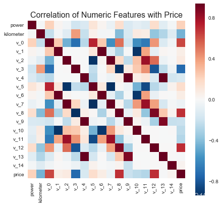
## 1) 相关性分析
price_numeric = Train_data[numeric_features]
correlation = price_numeric.corr()
print(correlation['price'].sort_values(ascending = False),'\n')

price        1.000000
v_12         0.692823
v_8          0.685798
v_0          0.628397
power        0.219834
v_5          0.164317
v_2          0.085322
v_6          0.068970
v_1          0.060914
v_14         0.035911
v_13        -0.013993
v_7         -0.053024
v_4         -0.147085
v_9         -0.206205
v_10        -0.246175
v_11        -0.275320
kilometer   -0.440519
v_3         -0.730946
Name: price, dtype: float64

f , ax = plt.subplots(figsize = (7, 7))

plt.title('Correlation of Numeric Features with Price',y=1,size=16)

sns.heatmap(correlation,square = True,  vmax=0.8)

<matplotlib.axes._subplots.AxesSubplot at 0x1f9584c33c8>

在这里插入图片描述

## 2) 查看几个特征得 偏度和峰值
for col in numeric_features:
    print('{:15}'.format(col), 
          'Skewness: {:05.2f}'.format(Train_data[col].skew()) , 
          '   ' ,
          'Kurtosis: {:06.2f}'.format(Train_data[col].kurt())  
         )

power           Skewness: 65.86     Kurtosis: 5733.45
kilometer       Skewness: -1.53     Kurtosis: 001.14
v_0             Skewness: -1.32     Kurtosis: 003.99
v_1             Skewness: 00.36     Kurtosis: -01.75
v_2             Skewness: 04.84     Kurtosis: 023.86
v_3             Skewness: 00.11     Kurtosis: -00.42
v_4             Skewness: 00.37     Kurtosis: -00.20
v_5             Skewness: -4.74     Kurtosis: 022.93
v_6             Skewness: 00.37     Kurtosis: -01.74
v_7             Skewness: 05.13     Kurtosis: 025.85
v_8             Skewness: 00.20     Kurtosis: -00.64
v_9             Skewness: 00.42     Kurtosis: -00.32
v_10            Skewness: 00.03     Kurtosis: -00.58
v_11            Skewness: 03.03     Kurtosis: 012.57
v_12            Skewness: 00.37     Kurtosis: 000.27
v_13            Skewness: 00.27     Kurtosis: -00.44
v_14            Skewness: -1.19     Kurtosis: 002.39
price           Skewness: 03.35     Kurtosis: 019.00

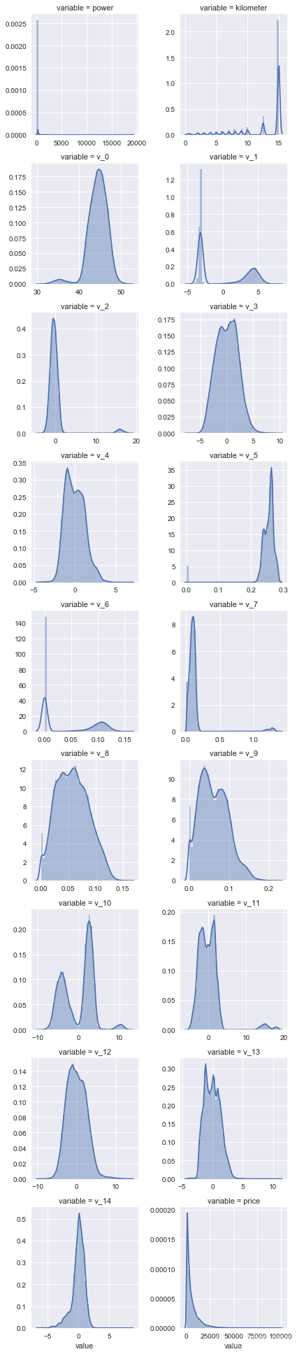
## 3) 每个数字特征得分布可视化
f = pd.melt(Train_data, value_vars=numeric_features)
g = sns.FacetGrid(f, col="variable",  col_wrap=2, sharex=False, sharey=False)
g = g.map(sns.distplot, "value")

在这里插入图片描述

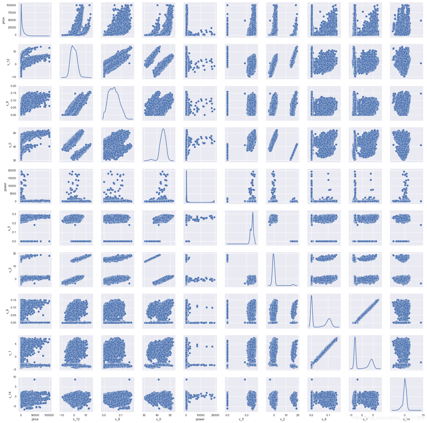
## 4) 数字特征相互之间的关系可视化
sns.set()
columns = ['price', 'v_12', 'v_8' , 'v_0', 'power', 'v_5',  'v_2', 'v_6', 'v_1', 'v_14']
sns.pairplot(Train_data[columns],size = 2 ,kind ='scatter',diag_kind='kde')
plt.show()

在这里插入图片描述

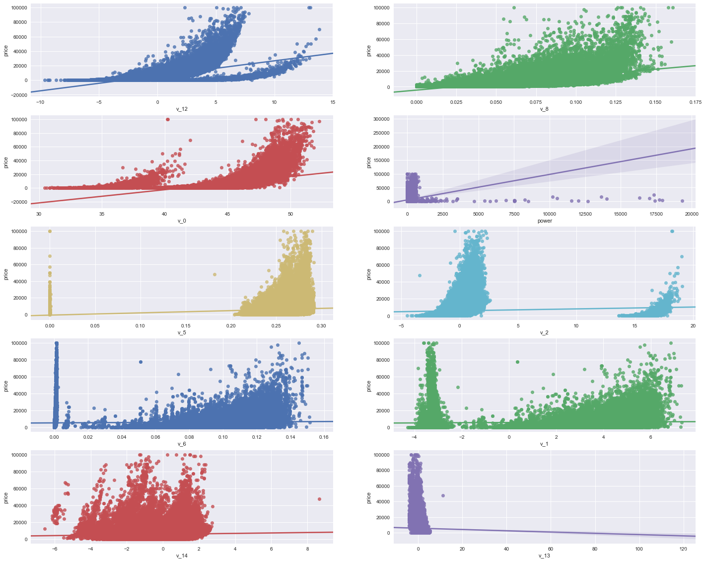
## 5) 多变量互相回归关系可视化
fig, ((ax1, ax2), (ax3, ax4), (ax5, ax6), (ax7, ax8), (ax9, ax10)) = plt.subplots(nrows=5, ncols=2, figsize=(24, 20))
# ['v_12', 'v_8' , 'v_0', 'power', 'v_5',  'v_2', 'v_6', 'v_1', 'v_14']
v_12_scatter_plot = pd.concat([Y_train,Train_data['v_12']],axis = 1)
sns.regplot(x='v_12',y = 'price', data = v_12_scatter_plot,scatter= True, fit_reg=True, ax=ax1)

v_8_scatter_plot = pd.concat([Y_train,Train_data['v_8']],axis = 1)
sns.regplot(x='v_8',y = 'price',data = v_8_scatter_plot,scatter= True, fit_reg=True, ax=ax2)

v_0_scatter_plot = pd.concat([Y_train,Train_data['v_0']],axis = 1)
sns.regplot(x='v_0',y = 'price',data = v_0_scatter_plot,scatter= True, fit_reg=True, ax=ax3)

power_scatter_plot = pd.concat([Y_train,Train_data['power']],axis = 1)
sns.regplot(x='power',y = 'price',data = power_scatter_plot,scatter= True, fit_reg=True, ax=ax4)

v_5_scatter_plot = pd.concat([Y_train,Train_data['v_5']],axis = 1)
sns.regplot(x='v_5',y = 'price',data = v_5_scatter_plot,scatter= True, fit_reg=True, ax=ax5)

v_2_scatter_plot = pd.concat([Y_train,Train_data['v_2']],axis = 1)
sns.regplot(x='v_2',y = 'price',data = v_2_scatter_plot,scatter= True, fit_reg=True, ax=ax6)

v_6_scatter_plot = pd.concat([Y_train,Train_data['v_6']],axis = 1)
sns.regplot(x='v_6',y = 'price',data = v_6_scatter_plot,scatter= True, fit_reg=True, ax=ax7)

v_1_scatter_plot = pd.concat([Y_train,Train_data['v_1']],axis = 1)
sns.regplot(x='v_1',y = 'price',data = v_1_scatter_plot,scatter= True, fit_reg=True, ax=ax8)

v_14_scatter_plot = pd.concat([Y_train,Train_data['v_14']],axis = 1)
sns.regplot(x='v_14',y = 'price',data = v_14_scatter_plot,scatter= True, fit_reg=True, ax=ax9)

v_13_scatter_plot = pd.concat([Y_train,Train_data['v_13']],axis = 1)
sns.regplot(x='v_13',y = 'price',data = v_13_scatter_plot,scatter= True, fit_reg=True, ax=ax10)

<matplotlib.axes._subplots.AxesSubplot at 0x1e1fac3a0b8>

在这里插入图片描述

## 1) unique分布
for fea in categorical_features:
    print(Train_data[fea].nunique())

categorical_features

['name',
 'model',
 'brand',
 'bodyType',
 'fuelType',
 'gearbox',
 'notRepairedDamage',
 'regionCode']

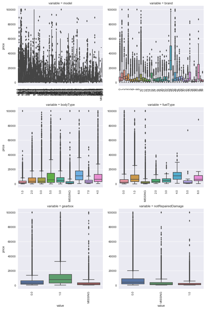
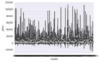
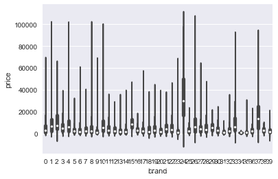
## 2) 类别特征箱形图可视化

# 因为 name和 regionCode的类别太稀疏了，这里我们把不稀疏的几类画一下
categorical_features = ['model',
 'brand',
 'bodyType',
 'fuelType',
 'gearbox',
 'notRepairedDamage']
for c in categorical_features:
    Train_data[c] = Train_data[c].astype('category')
    if Train_data[c].isnull().any():
        Train_data[c] = Train_data[c].cat.add_categories(['MISSING'])
        Train_data[c] = Train_data[c].fillna('MISSING')

def boxplot(x, y, **kwargs):
    sns.boxplot(x=x, y=y)
    x=plt.xticks(rotation=90)

f = pd.melt(Train_data, id_vars=['price'], value_vars=categorical_features)
g = sns.FacetGrid(f, col="variable",  col_wrap=2, sharex=False, sharey=False, size=5)
g = g.map(boxplot, "value", "price")

在这里插入图片描述

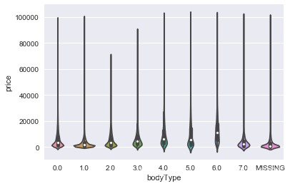
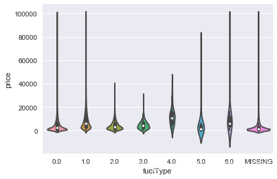
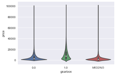
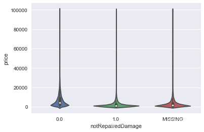
## 3) 类别特征的小提琴图可视化
catg_list = categorical_features
target = 'price'
for catg in catg_list :
    sns.violinplot(x=catg, y=target, data=Train_data)
    plt.show()

在这里插入图片描述

categorical_features = ['model',
 'brand',
 'bodyType',
 'fuelType',
 'gearbox',
 'notRepairedDamage']

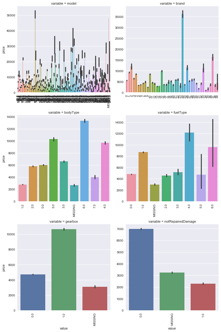
## 4) 类别特征的柱形图可视化
def bar_plot(x, y, **kwargs):
    sns.barplot(x=x, y=y)
    x=plt.xticks(rotation=90)

f = pd.melt(Train_data, id_vars=['price'], value_vars=categorical_features)
g = sns.FacetGrid(f, col="variable",  col_wrap=2, sharex=False, sharey=False, size=5)
g = g.map(bar_plot, "value", "price")

在这里插入图片描述

##  5) 类别特征的每个类别频数可视化(count_plot)
def count_plot(x,  **kwargs):
    sns.countplot(x=x)
    x=plt.xticks(rotation=90)

f = pd.melt(Train_data,  value_vars=categorical_features)
g = sns.FacetGrid(f, col="variable",  col_wrap=2, sharex=False, sharey=False, size=5)
g = g.map(count_plot, "value")

import pandas_profiling
pfr = pandas_profiling.ProfileReport(Train_data)
pfr.to_file("./example.html")#用pandas_profiling生成数据报告

qq_40791906

发布了3 篇原创文章 · 获赞 1 · 访问量 102

私信关注

猜你喜欢