数据挖掘——数据分析
根据提供的EDA代码打了遍(代码生成图上传麻烦,后面再上传),熟悉了下数据分析代码。晚上的直播总结。

2.1 EDA目标
- EDA的价值主要在于熟悉数据集,了解数据集,对数据集进行验证来确定所获得数据集可以用于接下来的机器学习或者深度学习使用。
- 当了解了数据集之后我们下一步就是要去了解变量间的相互关系以及变量与预测值之间的存在关系。
- 引导数据科学从业者进行数据处理以及特征工程的步骤,使数据集的结构和特征集让接下来的预测问题更加可靠。
- 完成对于数据的探索性分析,并对于数据进行一些图表或者文字总结并打卡。
2.2 内容介绍
- 载入各种数据科学以及可视化库:
- 数据科学库 pandas、numpy、scipy;
- 可视化库 matplotlib、seabon;
- 其他;
- 载入数据:
- 载入训练集和测试集;
- 简略观察数据(head()+shape);
- 数据总览:
- 通过describe()来熟悉数据的相关统计量
- 通过info()来熟悉数据类型
- 判断数据缺失和异常
- 查看每列的存在nan情况
- 异常值检测
- 了解预测值的分布
- 总体分布概况(无界约翰逊分布等)
- 查看skewness and kurtosis
- 查看预测值的具体频数
- 特征分为类别特征和数字特征,并对类别特征查看unique分布
- 数字特征分析
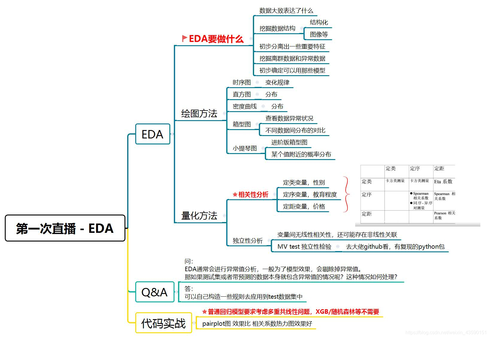
- 相关性分析
- 查看几个特征得 偏度和峰值
- 每个数字特征得分布可视化
- 数字特征相互之间的关系可视化
- 多变量互相回归关系可视化
- 类型特征分析
- unique分布
- 类别特征箱形图可视化
- 类别特征的小提琴图可视化
- 类别特征的柱形图可视化类别
- 特征的每个类别频数可视化(count_plot)
- 用pandas_profiling生成数据报告
2.3 代码示例
2.3.1 载入各种数据科学以及可视化库
以下库都是pip install 安装, 有特殊情况我会单独说明 例如 pip install pandas -i https://pypi.tuna.tsinghua.edu.cn/simple
#coding:utf-8
#导入warnings包,利用过滤器来实现忽略警告语句。
import warnings
warnings.filterwarnings('ignore')
import pandas as pd
import numpy as np
import matplotlib.pyplot as plt
import seaborn as sns
import missingno as msno
2.3.2 载入数据
## 1) 载入训练集和测试集; path = './datalab/231784/' Train_data = pd.read_csv(path+'used_car_train_20200313.csv', sep=' ') Test_data = pd.read_csv(path+'used_car_testA_20200313.csv', sep=' ')
所有特征集均脱敏处理(方便大家观看)
-
name - 汽车编码
-
regDate - 汽车注册时间
-
model - 车型编码
-
brand - 品牌
-
bodyType - 车身类型
扫描二维码关注公众号,回复: 10764200 查看本文章
-
fuelType - 燃油类型
-
gearbox - 变速箱
-
power - 汽车功率
-
kilometer - 汽车行驶公里
-
notRepairedDamage - 汽车有尚未修复的损坏
-
regionCode - 看车地区编码
-
seller - 销售方
-
offerType - 报价类型
-
creatDate - 广告发布时间
-
price - 汽车价格
-
v_0’, ‘v_1’, ‘v_2’, ‘v_3’, ‘v_4’, ‘v_5’, ‘v_6’, ‘v_7’, ‘v_8’, ‘v_9’, ‘v_10’, ‘v_11’, ‘v_12’, ‘v_13’,‘v_14’ 【匿名特征,包含v0-14在内15个匿名特征】
-
要养成看数据集的head()以及shape的习惯,这会让你每一步更放心,导致接下里的连串的错误, 如果对自己的pandas等操作不放心,建议执行一步看一下,这样会有效的方便你进行理解函数并进行操作
2.3.3 总览数据概况
-
describe种有每列的统计量,个数count、平均值mean、方差std、最小值min、中位数25% 50% 75% 、以及最大值 看这个信息主要是瞬间掌握数据的大概的范围以及每个值的异常值的判断,比如有的时候会发现999 9999 -1 等值这些其实都是nan的另外一种表达方式,有的时候需要注意下
-
info 通过info来了解数据每列的type,有助于了解是否存在除了nan以外的特殊符号异常
## 1) 通过describe()来熟悉数据的相关统计量Train_data.describe()[7]:
SaleID name regDate model brand bodyType fuelType gearbox power kilometer … v_5 v_6 v_7 v_8 v_9 v_10 v_11 v_12 v_13 v_14 count 150000.000000 150000.000000 1.500000e+05 149999.000000 150000.000000 145494.000000 141320.000000 144019.000000 150000.000000 150000.000000 … 150000.000000 150000.000000 150000.000000 150000.000000 150000.000000 150000.000000 150000.000000 150000.000000 150000.000000 150000.000000 mean 74999.500000 68349.172873 2.003417e+07 47.129021 8.052733 1.792369 0.375842 0.224943 119.316547 12.597160 … 0.248204 0.044923 0.124692 0.058144 0.061996 -0.001000 0.009035 0.004813 0.000313 -0.000688 std 43301.414527 61103.875095 5.364988e+04 49.536040 7.864956 1.760640 0.548677 0.417546 177.168419 3.919576 … 0.045804 0.051743 0.201410 0.029186 0.035692 3.772386 3.286071 2.517478 1.288988 1.038685 min 0.000000 0.000000 1.991000e+07 0.000000 0.000000 0.000000 0.000000 0.000000 0.000000 0.500000 … 0.000000 0.000000 0.000000 0.000000 0.000000 -9.168192 -5.558207 -9.639552 -4.153899 -6.546556 25% 37499.750000 11156.000000 1.999091e+07 10.000000 1.000000 0.000000 0.000000 0.000000 75.000000 12.500000 … 0.243615 0.000038 0.062474 0.035334 0.033930 -3.722303 -1.951543 -1.871846 -1.057789 -0.437034 50% 74999.500000 51638.000000 2.003091e+07 30.000000 6.000000 1.000000 0.000000 0.000000 110.000000 15.000000 … 0.257798 0.000812 0.095866 0.057014 0.058484 1.624076 -0.358053 -0.130753 -0.036245 0.141246 75% 112499.250000 118841.250000 2.007111e+07 66.000000 13.000000 3.000000 1.000000 0.000000 150.000000 15.000000 … 0.265297 0.102009 0.125243 0.079382 0.087491 2.844357 1.255022 1.776933 0.942813 0.680378 max 149999.000000 196812.000000 2.015121e+07 247.000000 39.000000 7.000000 6.000000 1.000000 19312.000000 15.000000 … 0.291838 0.151420 1.404936 0.160791 0.222787 12.357011 18.819042 13.847792 11.147669 8.658418 8 rows × 30 columns
Test_data.describe()[8]:
SaleID name regDate model brand bodyType fuelType gearbox power kilometer … v_5 v_6 v_7 v_8 v_9 v_10 v_11 v_12 v_13 v_14 count 50000.000000 50000.000000 5.000000e+04 50000.000000 50000.000000 48587.000000 47107.000000 48090.000000 50000.000000 50000.000000 … 50000.000000 50000.000000 50000.000000 50000.000000 50000.000000 50000.000000 50000.000000 50000.000000 50000.000000 50000.000000 mean 174999.500000 68542.223280 2.003393e+07 46.844520 8.056240 1.782185 0.373405 0.224350 119.883620 12.595580 … 0.248669 0.045021 0.122744 0.057997 0.062000 -0.017855 -0.013742 -0.013554 -0.003147 0.001516 std 14433.901067 61052.808133 5.368870e+04 49.469548 7.819477 1.760736 0.546442 0.417158 185.097387 3.908979 … 0.044601 0.051766 0.195972 0.029211 0.035653 3.747985 3.231258 2.515962 1.286597 1.027360 min 150000.000000 0.000000 1.991000e+07 0.000000 0.000000 0.000000 0.000000 0.000000 0.000000 0.500000 … 0.000000 0.000000 0.000000 0.000000 0.000000 -9.160049 -5.411964 -8.916949 -4.123333 -6.112667 25% 162499.750000 11203.500000 1.999091e+07 10.000000 1.000000 0.000000 0.000000 0.000000 75.000000 12.500000 … 0.243762 0.000044 0.062644 0.035084 0.033714 -3.700121 -1.971325 -1.876703 -1.060428 -0.437920 50% 174999.500000 52248.500000 2.003091e+07 29.000000 6.000000 1.000000 0.000000 0.000000 109.000000 15.000000 … 0.257877 0.000815 0.095828 0.057084 0.058764 1.613212 -0.355843 -0.142779 -0.035956 0.138799 75% 187499.250000 118856.500000 2.007110e+07 65.000000 13.000000 3.000000 1.000000 0.000000 150.000000 15.000000 … 0.265328 0.102025 0.125438 0.079077 0.087489 2.832708 1.262914 1.764335 0.941469 0.681163 max 199999.000000 196805.000000 2.015121e+07 246.000000 39.000000 7.000000 6.000000 1.000000 20000.000000 15.000000 … 0.291618 0.153265 1.358813 0.156355 0.214775 12.338872 18.856218 12.950498 5.913273 2.624622 8 rows × 29 columns
## 2) 通过info()来熟悉数据类型Train_data.info() <class 'pandas.core.frame.DataFrame'> RangeIndex: 150000 entries, 0 to 149999 Data columns (total 31 columns): SaleID 150000 non-null int64 name 150000 non-null int64 regDate 150000 non-null int64 model 149999 non-null float64 brand 150000 non-null int64 bodyType 145494 non-null float64 fuelType 141320 non-null float64 gearbox 144019 non-null float64 power 150000 non-null int64 kilometer 150000 non-null float64 notRepairedDamage 150000 non-null object regionCode 150000 non-null int64 seller 150000 non-null int64 offerType 150000 non-null int64 creatDate 150000 non-null int64 price 150000 non-null int64 v_0 150000 non-null float64 v_1 150000 non-null float64 v_2 150000 non-null float64 v_3 150000 non-null float64 v_4 150000 non-null float64 v_5 150000 non-null float64 v_6 150000 non-null float64 v_7 150000 non-null float64 v_8 150000 non-null float64 v_9 150000 non-null float64 v_10 150000 non-null float64 v_11 150000 non-null float64 v_12 150000 non-null float64 v_13 150000 non-null float64 v_14 150000 non-null float64 dtypes: float64(20), int64(10), object(1) memory usage: 35.5+ MBTest_data.info() <class 'pandas.core.frame.DataFrame'> RangeIndex: 50000 entries, 0 to 49999 Data columns (total 30 columns): SaleID 50000 non-null int64 name 50000 non-null int64 regDate 50000 non-null int64 model 50000 non-null float64 brand 50000 non-null int64 bodyType 48587 non-null float64 fuelType 47107 non-null float64 gearbox 48090 non-null float64 power 50000 non-null int64 kilometer 50000 non-null float64 notRepairedDamage 50000 non-null object regionCode 50000 non-null int64 seller 50000 non-null int64 offerType 50000 non-null int64 creatDate 50000 non-null int64 v_0 50000 non-null float64 v_1 50000 non-null float64 v_2 50000 non-null float64 v_3 50000 non-null float64 v_4 50000 non-null float64 v_5 50000 non-null float64 v_6 50000 non-null float64 v_7 50000 non-null float64 v_8 50000 non-null float64 v_9 50000 non-null float64 v_10 50000 non-null float64 v_11 50000 non-null float64 v_12 50000 non-null float64 v_13 50000 non-null float64 v_14 50000 non-null float64 dtypes: float64(20), int64(9), object(1) memory usage: 11.4+ MB2.3.4 判断数据缺失和异常
## 1) 查看每列的存在nan情况Train_data.isnull().sum()[11]:
SaleID 0 name 0 regDate 0 model 1 brand 0 bodyType 4506 fuelType 8680 gearbox 5981 power 0 kilometer 0 notRepairedDamage 0 regionCode 0 seller 0 offerType 0 creatDate 0 price 0 v_0 0 v_1 0 v_2 0 v_3 0 v_4 0 v_5 0 v_6 0 v_7 0 v_8 0 v_9 0 v_10 0 v_11 0 v_12 0 v_13 0 v_14 0 dtype: int64Test_data.isnull().sum()[12]:
SaleID                  0
name                    0
regDate                 0
model                   0
brand                   0
bodyType             1413
fuelType             2893
gearbox              1910
power                   0
kilometer               0
notRepairedDamage       0
regionCode              0
seller                  0
offerType               0
creatDate               0
v_0                     0
v_1                     0
v_2                     0
v_3                     0
v_4                     0
v_5                     0
v_6                     0
v_7                     0
v_8                     0
v_9                     0
v_10                    0
v_11                    0
v_12                    0
v_13                    0
v_14                    0
dtype: int64
# nan可视化missing = Train_data.isnull().sum()missing = missing[missing > 0]missing.sort_values(inplace=True)missing.plot.bar()[13]:
<matplotlib.axes._subplots.AxesSubplot at 0x7ff019312b38>通过以上两句可以很直观的了解哪些列存在 “nan”, 并可以把nan的个数打印,主要的目的在于 nan存在的个数是否真的很大,如果很小一般选择填充,如果使用lgb等树模型可以直接空缺,让树自己去优化,但如果nan存在的过多、可以考虑删掉
# 可视化看下缺省值msno.matrix(Train_data.sample(250))[14]:
<matplotlib.axes._subplots.AxesSubplot at 0x7ff019277198>msno.bar(Train_data.sample(1000))[15]:
<matplotlib.axes._subplots.AxesSubplot at 0x7ff0190fbda0># 可视化看下缺省值msno.matrix(Test_data.sample(250))[16]:
<matplotlib.axes._subplots.AxesSubplot at 0x7ff01698d4a8>msno.bar(Test_data.sample(1000))[17]:
<matplotlib.axes._subplots.AxesSubplot at 0x7ff0168d1f28>测试集的缺省和训练集的差不多情况, 可视化有四列有缺省,notRepairedDamage缺省得最多
## 2) 查看异常值检测Train_data.info() <class 'pandas.core.frame.DataFrame'> RangeIndex: 150000 entries, 0 to 149999 Data columns (total 31 columns): SaleID 150000 non-null int64 name 150000 non-null int64 regDate 150000 non-null int64 model 149999 non-null float64 brand 150000 non-null int64 bodyType 145494 non-null float64 fuelType 141320 non-null float64 gearbox 144019 non-null float64 power 150000 non-null int64 kilometer 150000 non-null float64 notRepairedDamage 150000 non-null object regionCode 150000 non-null int64 seller 150000 non-null int64 offerType 150000 non-null int64 creatDate 150000 non-null int64 price 150000 non-null int64 v_0 150000 non-null float64 v_1 150000 non-null float64 v_2 150000 non-null float64 v_3 150000 non-null float64 v_4 150000 non-null float64 v_5 150000 non-null float64 v_6 150000 non-null float64 v_7 150000 non-null float64 v_8 150000 non-null float64 v_9 150000 non-null float64 v_10 150000 non-null float64 v_11 150000 non-null float64 v_12 150000 non-null float64 v_13 150000 non-null float64 v_14 150000 non-null float64 dtypes: float64(20), int64(10), object(1) memory usage: 35.5+ MB可以发现除了notRepairedDamage 为object类型其他都为数字 这里我们把他的几个不同的值都进行显示就知道了
Train_data['notRepairedDamage'].value_counts()[20]:
0.0    111361
-       24324
1.0     14315
Name: notRepairedDamage, dtype: int64
可以看出来‘ - ’也为空缺值,因为很多模型对nan有直接的处理,这里我们先不做处理,先替换成nan
Train_data['notRepairedDamage'].replace('-', np.nan, inplace=True)Train_data['notRepairedDamage'].value_counts()[22]:
0.0 111361 1.0 14315 Name: notRepairedDamage, dtype: int64Train_data.isnull().sum()[23]:
SaleID 0 name 0 regDate 0 model 1 brand 0 bodyType 4506 fuelType 8680 gearbox 5981 power 0 kilometer 0 notRepairedDamage 24324 regionCode 0 seller 0 offerType 0 creatDate 0 price 0 v_0 0 v_1 0 v_2 0 v_3 0 v_4 0 v_5 0 v_6 0 v_7 0 v_8 0 v_9 0 v_10 0 v_11 0 v_12 0 v_13 0 v_14 0 dtype: int64Test_data['notRepairedDamage'].value_counts()[24]:
0.0    37249
-       8031
1.0     4720
Name: notRepairedDamage, dtype: int64
Test_data['notRepairedDamage'].replace('-', np.nan, inplace=True)以下两个类别特征严重倾斜,一般不会对预测有什么帮助,故这边先删掉,当然你也可以继续挖掘,但是一般意义不大
Train_data["seller"].value_counts()[26]:
0 149999 1 1 Name: seller, dtype: int64Train_data["offerType"].value_counts()[27]:
0    150000
Name: offerType, dtype: int64
del Train_data["seller"]del Train_data["offerType"]del Test_data["seller"]del Test_data["offerType"]2.3.5 了解预测值的分布
Train_data['price'][29]:
0 1850 1 3600 2 6222 3 2400 4 5200 5 8000 6 3500 7 1000 8 2850 9 650 10 3100 11 5450 12 1600 13 3100 14 6900 15 3200 16 10500 17 3700 18 790 19 1450 20 990 21 2800 22 350 23 599 24 9250 25 3650 26 2800 27 2399 28 4900 29 2999 ... 149970 900 149971 3400 149972 999 149973 3500 149974 4500 149975 3990 149976 1200 149977 330 149978 3350 149979 5000 149980 4350 149981 9000 149982 2000 149983 12000 149984 6700 149985 4200 149986 2800 149987 3000 149988 7500 149989 1150 149990 450 149991 24950 149992 950 149993 4399 149994 14780 149995 5900 149996 9500 149997 7500 149998 4999 149999 4700 Name: price, Length: 150000, dtype: int64Train_data['price'].value_counts()[30]:
500      2337
1500     2158
1200     1922
1000     1850
2500     1821
600      1535
3500     1533
800      1513
2000     1378
999      1356
750      1279
4500     1271
650      1257
1800     1223
2200     1201
850      1198
700      1174
900      1107
1300     1105
950      1104
3000     1098
1100     1079
5500     1079
1600     1074
300      1071
550      1042
350      1005
1250     1003
6500      973
1999      929
         ...
21560       1
7859        1
3120        1
2279        1
6066        1
6322        1
4275        1
10420       1
43300       1
305         1
1765        1
15970       1
44400       1
8885        1
2992        1
31850       1
15413       1
13495       1
9525        1
7270        1
13879       1
3760        1
24250       1
11360       1
10295       1
25321       1
8886        1
8801        1
37920       1
8188        1
Name: price, Length: 3763, dtype: int64
## 1) 总体分布概况(无界约翰逊分布等)import scipy.stats as sty = Train_data['price']plt.figure(1); plt.title('Johnson SU')sns.distplot(y, kde=False, fit=st.johnsonsu)plt.figure(2); plt.title('Normal')sns.distplot(y, kde=False, fit=st.norm)plt.figure(3); plt.title('Log Normal')sns.distplot(y, kde=False, fit=st.lognorm)[31]:
<matplotlib.axes._subplots.AxesSubplot at 0x7ff01668d278>
-
