@本文来源于公众号:csdn2299,喜欢可以关注公众号 程序员学府
这篇文章主要介绍了Python中利用LSTM模型进行时间序列预测分析的实现,文中通过示例代码介绍的非常详细,对大家的学习或者工作具有一定的参考学习价值,需要的朋友们下面随着小编来一起学习学习吧
时间序列模型
时间序列预测分析就是利用过去一段时间内某事件时间的特征来预测未来一段时间内该事件的特征。这是一类相对比较复杂的预测建模问题,和回归分析模型的预测不同,时间序列模型是依赖于事件发生的先后顺序的,同样大小的值改变顺序后输入模型产生的结果是不同的。
举个栗子:根据过去两年某股票的每天的股价数据推测之后一周的股价变化;根据过去2年某店铺每周想消费人数预测下周来店消费的人数等等
RNN 和 LSTM 模型
时间序列模型最常用最强大的的工具就是递归神经网络(recurrent neural network, RNN)。相比与普通神经网络的各计算结果之间相互独立的特点,RNN的每一次隐含层的计算结果都与当前输入以及上一次的隐含层结果相关。通过这种方法,RNN的计算结果便具备了记忆之前几次结果的特点。
典型的RNN网路结构如下: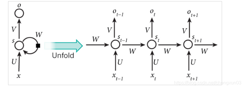
右侧为计算时便于理解记忆而产开的结构。简单说,x为输入层,o为输出层,s为隐含层,而t指第几次的计算;V,W,U为权重,其中计算第t次的隐含层状态时为St = f(UXt + WSt-1),实现当前输入结果与之前的计算挂钩的目的
RNN的局限:
由于RNN模型如果需要实现长期记忆的话需要将当前的隐含态的计算与前n次的计算挂钩,即St = f(UXt + W1St-1 + W2St-2 + … + WnSt-n),那样的话计算量会呈指数式增长,导致模型训练的时间大幅增加,因此RNN模型一般直接用来进行长期记忆计算。
LSTM模型
LSTM(Long Short-Term Memory)模型是一种RNN的变型,最早由Juergen Schmidhuber提出的。经典的LSTM模型结构如下: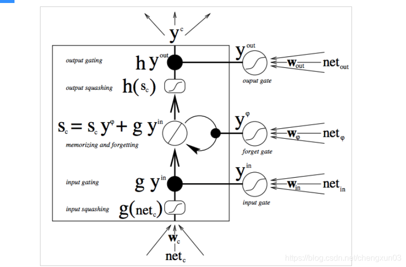
LSTM的特点就是在RNN结构以外添加了各层的阀门节点。阀门有3类:遗忘阀门(forget gate),输入阀门(input gate)和输出阀门(output gate)。这些阀门可以打开或关闭,用于将判断模型网络的记忆态(之前网络的状态)在该层输出的结果是否达到阈值从而加入到当前该层的计算中。如图中所示,阀门节点利用sigmoid函数将网络的记忆态作为输入计算;如果输出结果达到阈值则将该阀门输出与当前层的的计算结果相乘作为下一层的输入(PS:这里的相乘是在指矩阵中的逐元素相乘);如果没有达到阈值则将该输出结果遗忘掉。每一层包括阀门节点的权重都会在每一次模型反向传播训练过程中更新。更具体的LSTM的判断计算过程如下图所示: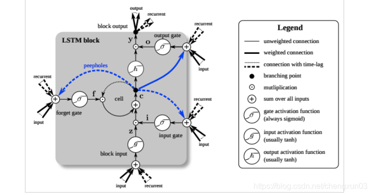
LSTM模型的记忆功能就是由这些阀门节点实现的。当阀门打开的时候,前面模型的训练结果就会关联到当前的模型计算,而当阀门关闭的时候之前的计算结果就不再影响当前的计算。因此,通过调节阀门的开关我们就可以实现早期序列对最终结果的影响。而当你不不希望之前结果对之后产生影响,比如自然语言处理中的开始分析新段落或新章节,那么把阀门关掉即可
下图具体演示了阀门是如何工作的:通过阀门控制使序列第1的输入的变量影响到了序列第4,6的的变量计算结果。
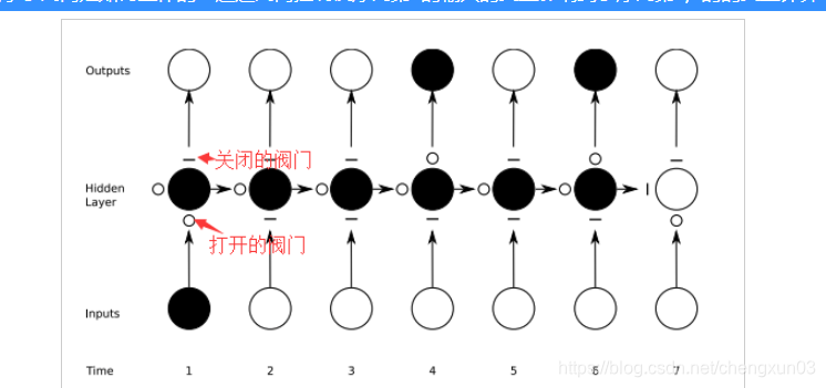
黑色实心圆代表对该节点的计算结果输出到下一层或下一次计算;空心圆则表示该节点的计算结果没有输入到网络或者没有从上一次收到信号。
Python中实现LSTM模型搭建
Python中有不少包可以直接调用来构建LSTM模型,比如pybrain, kears, tensorflow, cikit-neuralnetwork等
这里我们选用keras。(PS:如果操作系统用的linux或者mac,强推Tensorflow!!!)
因为LSTM神经网络模型的训练可以通过调整很多参数来优化,例如activation函数,LSTM层数,输入输出的变量维度等,调节过程相当复杂。这里只举一个最简单的应用例子来描述LSTM的搭建过程。
应用实例
基于某家店的某顾客的历史消费的时间推测该顾客前下次来店的时间。具体数据如下所示:
消费时间
2015-05-15 14:03:51
2015-05-15 15:32:46
2015-06-28 18:00:17
2015-07-16 21:27:18
2015-07-16 22:04:51
2015-09-08 14:59:56
..
..
具体操作:
- 原始数据转化
首先需要将时间点数据进行数值化。将具体时间转化为时间段用于表示该用户相邻两次消费的时间间隔,然后再导入模型进行训练是比较常用的手段。转化后的数据如下:
消费间隔
0
44
18
0
54
..
..
2.生成模型训练数据集(确定训练集的窗口长度)
这里的窗口指需要几次消费间隔用来预测下一次的消费间隔。这里我们先采用窗口长度为3, 即用t-2, t-1,t次的消费间隔进行模型训练,然后用t+1次间隔对结果进行验证。数据集格式如下:X为训练数据,Y为验证数据。
PS: 这里说确定也不太合适,因为窗口长度需要根据模型验证结果进行调整的。
X1  X2  X3  Y
0  44  18  0
44  18  0  54
..
..
注:直接这样预测一般精度会比较差,可以把预测值Y根据数值bin到几类,然后用转换成one-hot标签再来训练会比较好。比如如果把Y按数值范围分到五类(1:0-20,2:20-40,3:40-60,4:60-80,5:80-100)上式可化为:
X1  X2  X3  Y
0  44  18  0
44  18  0  4
...
Y转化成one-hot以后则是
1  0  0  0  0
0  0  0  0  1
...
- 网络模型结构的确定和调整
这里我们使用python的keras库。(用java的同学可以参考下deeplearning4j这个库)。网络的训练过程设计到许多参数的调整:比如
需要确定LSTM模块的激活函数(activation fucntion)(keras中默认的是tanh);
确定接收LSTM输出的完全连接人工神经网络(fully-connected artificial neural network)的激活函数(keras中默认为linear);
确定每一层网络节点的舍弃率(为了防止过度拟合(overfit)),这里我们默认值设定为0.2;
确定误差的计算方式,这里我们使用均方误差(mean squared error);
确定权重参数的迭代更新方式,这里我们采用RMSprop算法,通常用于RNN网络。确定模型训练的epoch和batch size
一般来说LSTM模块的层数越多(一般不超过3层,再多训练的时候就比较难收敛),对高级别的时间表示的学习能力越强;同时,最后会加一层普通的神经网路层用于输出结果的降维。典型结构如下: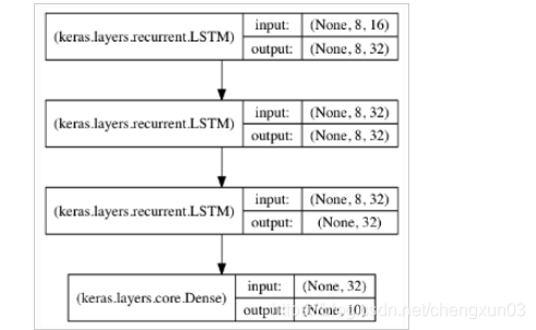
如果需要将多个序列进行同一个模型的训练,可以将序列分别输入到独立的LSTM模块然后输出结果合并后输入到普通层。结构如下: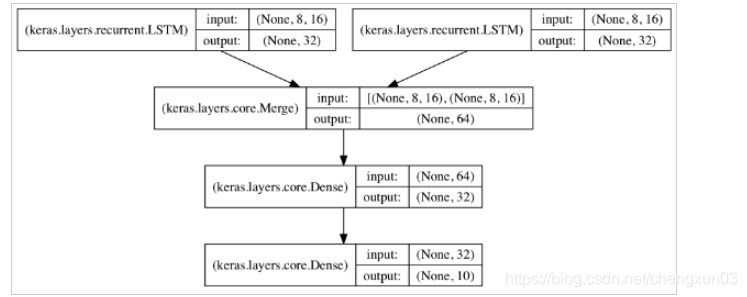
4. 模型训练和结果预测
将上述数据集按4:1的比例随机拆分为训练集和验证集,这是为了防止过度拟合。训练模型。然后将数据的X列作为参数导入模型便可得到预测值,与实际的Y值相比便可得到该模型的优劣。
实现代码
时间间隔序列格式化成所需的训练集格式
import pandas as pd
import numpy as np

def create_interval_dataset(dataset, look_back):
  """
  :param dataset: input array of time intervals
  :param look_back: each training set feature length
  :return: convert an array of values into a dataset matrix.
  """
  dataX, dataY = [], []
  for i in range(len(dataset) - look_back):
    dataX.append(dataset[i:i+look_back])
    dataY.append(dataset[i+look_back])
  return np.asarray(dataX), np.asarray(dataY)

df = pd.read_csv("path-to-your-time-interval-file")
dataset_init = np.asarray(df)  # if only 1 column
dataX, dataY = create_interval_dataset(dataset, lookback=3)  # look back if the training set sequence length
这里的输入数据来源是csv文件,如果输入数据是来自数据库的话可以参考这里
LSTM网络结构搭建
import pandas as pd
import numpy as np
import random
from keras.models import Sequential, model_from_json
from keras.layers import Dense, LSTM, Dropout

class NeuralNetwork():
  def __init__(self, **kwargs):
    """
    :param **kwargs: output_dim=4: output dimension of LSTM layer; activation_lstm='tanh': activation function for LSTM layers; activation_dense='relu': activation function for Dense layer; activation_last='sigmoid': activation function for last layer; drop_out=0.2: fraction of input units to drop; np_epoch=10, the number of epoches to train the model. epoch is one forward pass and one backward pass of all the training examples; batch_size=32: number of samples per gradient update. The higher the batch size, the more memory space you'll need; loss='mean_square_error': loss function; optimizer='rmsprop'
    """
    self.output_dim = kwargs.get('output_dim', 8)
    self.activation_lstm = kwargs.get('activation_lstm', 'relu')
    self.activation_dense = kwargs.get('activation_dense', 'relu')
    self.activation_last = kwargs.get('activation_last', 'softmax')  # softmax for multiple output
    self.dense_layer = kwargs.get('dense_layer', 2)   # at least 2 layers
    self.lstm_layer = kwargs.get('lstm_layer', 2)
    self.drop_out = kwargs.get('drop_out', 0.2)
    self.nb_epoch = kwargs.get('nb_epoch', 10)
    self.batch_size = kwargs.get('batch_size', 100)
    self.loss = kwargs.get('loss', 'categorical_crossentropy')
    self.optimizer = kwargs.get('optimizer', 'rmsprop')

    def NN_model(self, trainX, trainY, testX, testY):
    """
    :param trainX: training data set
    :param trainY: expect value of training data
    :param testX: test data set
    :param testY: epect value of test data
    :return: model after training
    """
    print "Training model is LSTM network!"
    input_dim = trainX[1].shape[1]
    output_dim = trainY.shape[1] # one-hot label
    # print predefined parameters of current model:
    model = Sequential()
    # applying a LSTM layer with x dim output and y dim input. Use dropout parameter to avoid overfitting
    model.add(LSTM(output_dim=self.output_dim,
            input_dim=input_dim,
            activation=self.activation_lstm,
            dropout_U=self.drop_out,
            return_sequences=True))
    for i in range(self.lstm_layer-2):
      model.add(LSTM(output_dim=self.output_dim,
            input_dim=self.output_dim,
            activation=self.activation_lstm,
            dropout_U=self.drop_out,
            return_sequences=True))
    # argument return_sequences should be false in last lstm layer to avoid input dimension incompatibility with dense layer
    model.add(LSTM(output_dim=self.output_dim,
            input_dim=self.output_dim,
            activation=self.activation_lstm,
            dropout_U=self.drop_out))
    for i in range(self.dense_layer-1):
      model.add(Dense(output_dim=self.output_dim,
            activation=self.activation_last))
    model.add(Dense(output_dim=output_dim,
            input_dim=self.output_dim,
            activation=self.activation_last))
    # configure the learning process
    model.compile(loss=self.loss, optimizer=self.optimizer, metrics=['accuracy'])
    # train the model with fixed number of epoches
    model.fit(x=trainX, y=trainY, nb_epoch=self.nb_epoch, batch_size=self.batch_size, validation_data=(testX, testY))
    # store model to json file
    model_json = model.to_json()
    with open(model_path, "w") as json_file:
      json_file.write(model_json)
    # store model weights to hdf5 file
    if model_weight_path:
      if os.path.exists(model_weight_path):
        os.remove(model_weight_path)
      model.save_weights(model_weight_path) # eg: model_weight.h5
    return model
这里写的只涉及LSTM网络的结构搭建,至于如何把数据处理规范化成网络所需的结构以及把模型预测结果与实际值比较统计的可视化,就需要根据实际情况做调整了
非常感谢你的阅读
大学的时候选择了自学python,工作了发现吃了计算机基础不好的亏,学历不行这是
没办法的事,只能后天弥补,于是在编码之外开启了自己的逆袭之路,不断的学习python核心知识,深入的研习计算机基础知识,整理好了,如果你也不甘平庸,那就与我一起在编码之外,不断成长吧!
其实这里不仅有技术,更有那些技术之外的东西,比如,如何做一个精致的程序员,而不是“屌丝”,程序员本身就是高贵的一种存在啊,难道不是吗?[点击加入]想做你自己想成为高尚人,加油!
