tensorflow下用LSTM网络进行时间序列预测

引言：

最近，一直在看关于时间序列预测这一方面的东西。在这里总结一下：

1.时间序列分析常用的模型有AR,MA,ARIMA,以及RNN和LSTM

2.大多数预测模型都能做时间序列分析（主要是如何将已知问题转化为带有时间戳的序列问题）

参考：如何将时间序列转换为Python中的监督学习问题（1）

3.我们常说的预测我总结出来有两层含义：

（1）目前我查资料遇到最多的“预测”：实际上就是做曲线拟合，根据一部分数据进行建模（拟合曲线），然后用另一部分数据对所建的模型进行测试（看测试点与曲线的偏离程度）。也就是实时分析（适合跟据多变量来预测单变量或者多变量）比如：预测某一发电机的发电量。

（2）我所理解的预测：根据历史数据来预测未来的数据（未来所有数据是不可知的）比如：股票的走势。

总的来说：我认为时间序列分析问题分为两种情况1.无监督问题2.有监督问题3.两者的相互转化

转化问题参考：如何将时间序列转换为Python中的监督学习问题（1）

接下来就先说第一种预测：

介绍tensorflow下用LSTM网络进行时间序列预测。首先要说的是分为1.单层LSTM预测单变量或多变量2.多层LSTM预测单变量或多变量。本文只介绍多层LSTM预测多变量：

本数据是股票的数据，结果可能效果不好，有需要的话可以自己调试一下，主要是记录一下思路。

#！/usr/bin/env python
# encoding: utf-8
'''
@author: 真梦行路
@file: tf_lstm2.py
@time: 2018/8/13 11:27
'''
###引入第三方模块###
import numpy as np
import matplotlib.pyplot as plt
import tensorflow as tf
import os
import pandas as pd

###读取数据###
df=pd.read_csv(os.getcwd()+'\\data\\dataset_2.csv')
data=df.iloc[:,2:10].values
###定义设置LSTM常量###
rnn_unit=20    #隐层单元的数量
input_size=6   #输入矩阵维度
output_size=2  #输出矩阵维度
lr=0.0006      #学习率
time_step=20   #设置时间步长
###制作带时间步长的训练集###
def get_train_data(batch_size=60,time_step=15,train_begin=0,train_end=5800):
    batch_index=[]
    data_train=data[train_begin:train_end]
    normalized_train_data=(data_train-np.mean(data_train,axis=0))/np.std(data_train,axis=0)  #标准化
    train_x,train_y=[],[]   #训练集
    for i in range(len(normalized_train_data)-time_step):
       if i % batch_size==0:
           batch_index.append(i)
       x=normalized_train_data[i:i+time_step,:6]
       y=normalized_train_data[i:i+time_step,6:]
       train_x.append(x.tolist())
       train_y.append(y.tolist())
    batch_index.append((len(normalized_train_data)-time_step))
    return batch_index,train_x,train_y

###制作带时间步长的测试集###
def get_test_data(time_step=15,test_begin=5800):
    data_test=data[test_begin:]
    mean=np.mean(data_test,axis=0)
    std=np.std(data_test,axis=0)
    normalized_test_data=(data_test-mean)/std  #标准化
    size=(len(normalized_test_data)+time_step-1)//time_step  #有size个sample
    test_x,test_y=[],[]
    for i in range(size-1):
       x=normalized_test_data[i*time_step:(i+1)*time_step,:6]
       y=normalized_test_data[i*time_step:(i+1)*time_step,6:]
       test_x.append(x.tolist())
       test_y.extend(y)
    test_x.append((normalized_test_data[(i+1)*time_step:,:6]).tolist())
    test_y.extend((normalized_test_data[(i+1)*time_step:,6:]).tolist())
    return mean,std,test_x,test_y
#——————————————————定义LSTM网络权重和偏置——————————————————
#输入层、输出层权重、偏置

weights={
         'in':tf.Variable(tf.random_normal([input_size,rnn_unit])),
         'out':tf.Variable(tf.random_normal([rnn_unit,2]))
        }
biases={
        'in':tf.Variable(tf.constant(0.1,shape=[rnn_unit,])),
        'out':tf.Variable(tf.constant(0.1,shape=[2,]))
       }

#——————————————————定义LSTM网络——————————————————
def lstm(X):
    batch_size=tf.shape(X)[0]
    time_step=tf.shape(X)[1]
    w_in=weights['in']
    b_in=biases['in']
    input=tf.reshape(X,[-1,input_size])  #需要将tensor转成2维进行计算，计算后的结果作为隐藏层的输入
    input_rnn=tf.matmul(input,w_in)+b_in
    input_rnn=tf.reshape(input_rnn,[-1,time_step,rnn_unit])  #将tensor转成3维，作为lstm cell的输入
    cell1=tf.nn.rnn_cell.BasicLSTMCell(rnn_unit)
    cell2=tf.nn.rnn_cell.BasicLSTMCell(rnn_unit)
    cell=tf.nn.rnn_cell.MultiRNNCell(cells=[cell1,cell2])
    init_state=cell.zero_state(batch_size,dtype=tf.float32)
    with tf.variable_scope('scope', reuse=tf.AUTO_REUSE):
        output_rnn,final_states=tf.nn.dynamic_rnn(cell, input_rnn,initial_state=init_state, dtype=tf.float32)  #output_rnn是记录lstm每个输出节点的结果，final_states是最后一个cell的结果
    output=tf.reshape(output_rnn,[-1,rnn_unit]) #作为输出层的输入
    w_out=weights['out']
    b_out=biases['out']
    pred=tf.matmul(output,w_out)+b_out
    return pred,final_states

#——————————————————LSTM模型训练——————————————————
def train_lstm(batch_size=60,time_step=15,train_begin=2000,train_end=5800):
    X=tf.placeholder(tf.float32, shape=[None,time_step,input_size])
    Y=tf.placeholder(tf.float32, shape=[None,time_step,output_size])
    batch_index,train_x,train_y=get_train_data(batch_size,time_step,train_begin,train_end)
    pred,_=lstm(X)
    ###损失函数###
    loss=tf.reduce_mean(tf.square(tf.reshape(pred,[-1,2])-tf.reshape(Y, [-1,2])))
    train_op=tf.train.AdamOptimizer(lr).minimize(loss)
    saver=tf.train.Saver(tf.global_variables(),max_to_keep=4)#只保留最后4次的模型参数
    # module_file = tf.train.latest_checkpoint(os.getcwd()+'\\data\\module')
    with tf.Session() as sess:
        sess.run(tf.global_variables_initializer())
        # saver.restore(sess, module_file)
        #重复训练10000次
        for i in range(11):
            for step in range(len(batch_index)-1):
                _,loss_=sess.run([train_op,loss],feed_dict={X:train_x[batch_index[step]:batch_index[step+1]],Y:train_y[batch_index[step]:batch_index[step+1]]})
            print(i,loss_)
            if i % 10==0:
                print("保存模型：",saver.save(sess,os.getcwd()+'\\data\\module\\stock2.mode2',global_step=i))
#————————————————LSTM模型预测————————————————————
def prediction(time_step=15):
    X=tf.placeholder(tf.float32, shape=[None,time_step,input_size])#创建输入流图
    Y=tf.placeholder(tf.float32, shape=[None,time_step,output_size])#创建输出流图
    mean,std,test_x,test_y=get_test_data(time_step)
    pred,_=lstm(X)
    saver=tf.train.Saver(tf.global_variables())
    with tf.Session() as sess:
        ###参数恢复，调用已经训练好的模型###
        module_file = tf.train.latest_checkpoint(os.getcwd()+'\\data\\module')
        saver.restore(sess, module_file)
        test_predict=[]
        for step in range(len(test_x)-1):
          prob=sess.run(pred,feed_dict={X:[test_x[step]]})
          predict=prob.reshape(-1,1)
          test_predict.extend(predict)

        ###循环输出其中一个预测变量###
        predict_test=[]
        for i in range(len(test_predict)):
            if i%2==0:
                predict_test.append(test_predict[i])
        ###循环输出测试原始数据###
        y_test=[]
        test_y=np.array(test_y).reshape(-1,1)
        for i in range(len(test_y)):
            if i%2==0:
                y_test.append(test_y[i])
        ###数据反归一化###
        test_y=np.array(y_test)*std[6]+mean[6]
        test_predict=np.array(predict_test)*std[6]+mean[6]
        acc=np.average(np.abs(test_predict-test_y[:len(test_predict)])/test_y[:len(test_predict)])  #偏差
        print(acc)
        #以折线图表示结果
        plt.figure()
        plt.plot(list(range(len(test_predict))), test_predict, color='b')
        plt.plot(list(range(len(test_y))), test_y,  color='r')
        plt.show()
train_lstm()
prediction()

结果图：

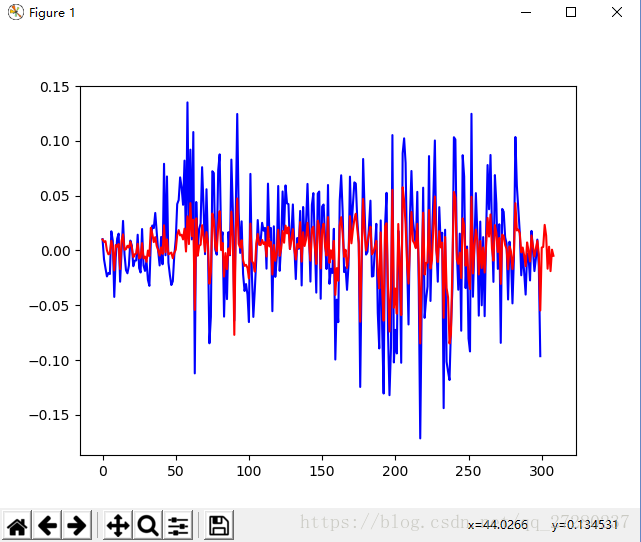
从图中可以看出，曲线的走势已经大致的描述出来了，但是画出的幅度比较大。 

第二种预测： 

介绍单层LSTM预测单变量。

#！/usr/bin/env python
# encoding: utf-8
'''
@author: 真梦行路
@file: tf_lstm.py
@time: 2018/8/9 17:11
'''
import pandas as pd
import numpy as np
import matplotlib.pyplot as plt
import tensorflow as tf
import os

df=pd.read_csv(os.getcwd()+'\\data\\dataset_1.csv',encoding='gbk')
data=np.array(df['最高价'])
data=data[::-1]

plt.figure()
plt.plot(data)
normalize_data=(data-np.mean(data))/np.std(data)
normalize_data=normalize_data[:,np.newaxis]

time_step=20
rnn_unit=10
batch_size=60
input_size=1
output_size=1
lr=0.0006
train_x,train_y=[],[]

for i in range(len(normalize_data)-time_step-1):
    x=normalize_data[i:i+time_step]
    y=normalize_data[i+1:i+time_step+1]
    train_x.append(x.tolist())
    train_y.append(y.tolist())

X=tf.placeholder(tf.float32, [None,time_step,input_size])
Y=tf.placeholder(tf.float32, [None,time_step,output_size])
#
weights={
         'in':tf.Variable(tf.random_normal([input_size,rnn_unit])),
         'out':tf.Variable(tf.random_normal([rnn_unit,1]))
         }
biases={
        'in':tf.Variable(tf.constant(0.1,shape=[rnn_unit,])),
        'out':tf.Variable(tf.constant(0.1,shape=[1,]))
        }

def lstm(batch):      #
    w_in=weights['in']
    b_in=biases['in']
    input=tf.reshape(X,[-1,input_size])  #
    input_rnn=tf.matmul(input,w_in)+b_in
    input_rnn=tf.reshape(input_rnn,[-1,time_step,rnn_unit])  #
    cell=tf.nn.rnn_cell.BasicLSTMCell(rnn_unit)
    init_state=cell.zero_state(batch,dtype=tf.float32)
    with tf.variable_scope('scope', reuse=tf.AUTO_REUSE):
        output_rnn,final_states=tf.nn.dynamic_rnn(cell, input_rnn,initial_state=init_state, dtype=tf.float32)
    output=tf.reshape(output_rnn,[-1,rnn_unit]) #
    w_out=weights['out']
    b_out=biases['out']
    pred=tf.matmul(output,w_out)+b_out
    return pred,final_states
def train_lstm():
    global batch_size
    pred,_=lstm(batch_size)
    loss=tf.reduce_mean(tf.square(tf.reshape(pred,[-1])-tf.reshape(Y, [-1])))
    train_op=tf.train.AdamOptimizer(lr).minimize(loss)
    saver=tf.train.Saver(tf.global_variables())
    with tf.Session() as sess:
        sess.run(tf.global_variables_initializer())
        for i in range(101):
            step=0
            start=0
            end=start+batch_size
            while(end<len(train_x)):
                _,loss_=sess.run([train_op,loss],feed_dict={X:train_x[start:end],Y:train_y[start:end]})
                start+=batch_size
                end=start+batch_size
                if step%10==0:
                    print(i,step,loss_)
                    print("保存模型：", saver.save(sess,os.getcwd()+'\\data\\module\\stock1.model', global_step=i))
                step+=1
def prediction():
    pred,_=lstm(1)      #
    saver=tf.train.Saver(tf.global_variables())
    with tf.Session() as sess:
        module_file = tf.train.latest_checkpoint(os.getcwd()+'\\data\\module')
        saver.restore(sess, module_file)
        prev_seq=train_x[-1]
        predict=[]
        for i in range(10): #往后预测10个数据
            next_seq=sess.run(pred,feed_dict={X:[prev_seq]})
            predict.append(next_seq[-1])
            prev_seq=np.vstack((prev_seq[1:],next_seq[-1]))
        plt.figure()
        plt.plot(list(range(len(normalize_data))), normalize_data, color='b')
        plt.plot(list(range(len(normalize_data), len(normalize_data) + len(predict))), predict, color='r')
        plt.show()

train_lstm()
prediction()

结果图：

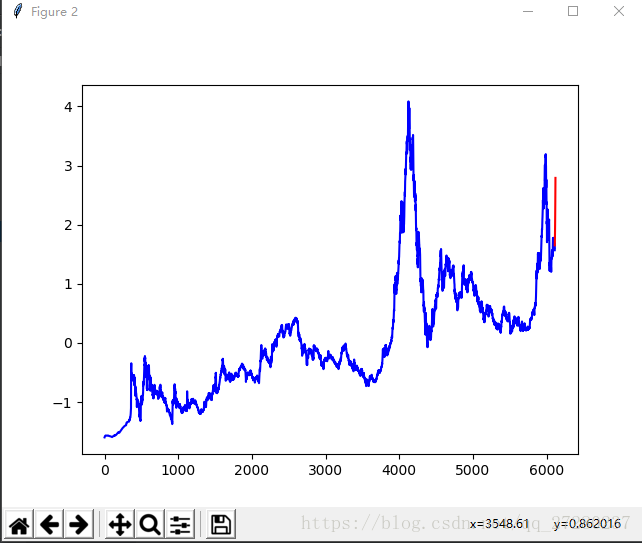
从图中可以看出，确实是已经往后预测出了10个点。但是精度不够，我训练了101次训练的次数有点少，大家可以尝试1000次甚至更多（注：此图是标准化后的数据，程序中并没有反标准化）

本文的完整程序以及数据集下载在这里。