《BP神经网络的MATLAB实现》

- 一 BP神经网络实现不使用MATLAB神经网络工具箱
- 二使用MATLAB的神经网络工具箱简易实现BP网络

一. BP神经网络实现（不使用MATLAB神经网络工具箱）

1. 问题

公路运量主要包括公路客运量和公路货运量两方面。某个地区的公路运量主要与该地区的人数、机动车数量和公路面积有关，已知该地区20年(1990-2009)的公路运量相关数据如下：

人数/万人

20.55 22.44 25.37 27.13 29.45 30.10 30.96 34.06 36.42 38.09 39.13 39.99 41.93 44.59 47.30 52.89 55.73 56.76 59.17 60.63

机动车数量/万辆

0.6 0.75 0.85 0.9 1.05 1.35 1.45 1.6 1.7 1.85 2.15 2.2 2.25 2.35 2.5 2.6 2.7 2.85 2.95 3.1

公路面积/单位：万平方公里

0.09 0.11 0.11 0.14 0.20 0.23 0.23 0.32 0.32 0.34 0.36 0.36 0.38 0.49 0.56 0.59 0.59 0.67 0.69 0.79

公路客运量/万人

5126 6217 7730 9145 10460 11387 12353 15750 18304 19836 21024 19490 20433 22598 25107 33442 36836 40548 42927 43462

公路货运量/万吨

1237 1379 1385 1399 1663 1714 1834 4322 8132 8936 11099 11203 10524 11115 13320 16762 18673 20724 20803 21804

2. 分析

样本数据较多，且已知影响数据的因素（三大因素：该地区的人数、机动车数量和公路面积），可考虑将其作为BP神经网络的训练集，对该神经网络进行训练，然后对训练好的神经网络进行测试，最后使用测试合格的神经网络进行预测工作。

3. MATLAB实现代码

BP_road.m

numberOfSample = 20; %输入样本数量
%取测试样本数量等于输入(训练集)样本数量，因为输入样本（训练集）容量较少，否则一般必须用新鲜数据进行测试
numberOfTestSample = 20; 
numberOfForcastSample = 2; 
numberOfHiddenNeure = 8;
inputDimension = 3;
outputDimension = 2;


%准备好训练集

%人数(单位：万人)
numberOfPeople=[20.55 22.44 25.37 27.13 29.45 30.10 30.96 34.06 36.42 38.09 39.13 39.99 41.93 44.59 47.30 52.89 55.73 56.76 59.17 60.63];
%机动车数(单位：万辆)
numberOfAutomobile=[0.6 0.75 0.85 0.9 1.05 1.35 1.45 1.6 1.7 1.85 2.15 2.2 2.25 2.35 2.5 2.6 2.7 2.85 2.95 3.1];
%公路面积(单位：万平方公里)
roadArea=[0.09 0.11 0.11 0.14 0.20 0.23 0.23 0.32 0.32 0.34 0.36 0.36 0.38 0.49 0.56 0.59 0.59 0.67 0.69 0.79];
%公路客运量(单位：万人)
passengerVolume = [5126 6217 7730 9145 10460 11387 12353 15750 18304 19836 21024 19490 20433 22598 25107 33442 36836 40548 42927 43462];
%公路货运量(单位：万吨)
freightVolume = [1237 1379 1385 1399 1663 1714 1834 4322 8132 8936 11099 11203 10524 11115 13320 16762 18673 20724 20803 21804];

%由系统时钟种子产生随机数
rand('state', sum(100*clock));

%输入数据矩阵
input = [numberOfPeople; numberOfAutomobile; roadArea];
%目标（输出）数据矩阵
output = [passengerVolume; freightVolume];

%对训练集中的输入数据矩阵和目标数据矩阵进行归一化处理
[sampleInput, minp, maxp, tmp, mint, maxt] = premnmx(input, output);

%噪声强度
noiseIntensity = 0.01;
%利用正态分布产生噪声
noise = noiseIntensity * randn(outputDimension, numberOfSample);
%给样本输出矩阵tmp添加噪声，防止网络过度拟合
sampleOutput = tmp + noise;

%取测试样本输入(输出)与输入样本相同，因为输入样本（训练集）容量较少，否则一般必须用新鲜数据进行测试
testSampleInput = sampleInput;
testSampleOutput = sampleOutput;

%最大训练次数
maxEpochs = 50000;

%网络的学习速率
learningRate = 0.035;

%训练网络所要达到的目标误差
error0 = 0.65*10^(-3);

%初始化输入层与隐含层之间的权值
W1 = 0.5 * rand(numberOfHiddenNeure, inputDimension) - 0.1;
%初始化输入层与隐含层之间的阈值
B1 = 0.5 * rand(numberOfHiddenNeure, 1) - 0.1;
%初始化输出层与隐含层之间的权值
W2 = 0.5 * rand(outputDimension, numberOfHiddenNeure) - 0.1;
%初始化输出层与隐含层之间的阈值
B2 = 0.5 * rand(outputDimension, 1) - 0.1;

%保存能量函数(误差平方和)的历史记录
errorHistory = [];

for i = 1:maxEpochs
    %隐含层输出
    hiddenOutput = logsig(W1 * sampleInput + repmat(B1, 1, numberOfSample));
    %输出层输出
    networkOutput = W2 * hiddenOutput + repmat(B2, 1, numberOfSample);
    %实际输出与网络输出之差
    error = sampleOutput - networkOutput;
    %计算能量函数(误差平方和)
    E = sumsqr(error);
    errorHistory = [errorHistory E];

    if E < error0
        break;
    end

    %以下依据能量函数的负梯度下降原理对权值和阈值进行调整
    delta2 = error;
    delta1 = W2' * delta2.*hiddenOutput.*(1 - hiddenOutput);

    dW2 = delta2 * hiddenOutput';
    dB2 = delta2 * ones(numberOfSample, 1);

    dW1 = delta1 * sampleInput';
    dB1 = delta1 * ones(numberOfSample, 1);

    W2 = W2 + learningRate * dW2;
    B2 = B2 + learningRate * dB2;

    W1 = W1 + learningRate * dW1;
    B1 = B1 + learningRate * dB1;
end

%下面对已经训练好的网络进行(仿真)测试

%对测试样本进行处理
testHiddenOutput = logsig(W1 * testSampleInput + repmat(B1, 1, numberOfTestSample));
testNetworkOutput =  W2 * testHiddenOutput + repmat(B2, 1, numberOfTestSample);
%还原网络输出层的结果(反归一化)
a = postmnmx(testNetworkOutput, mint, maxt);

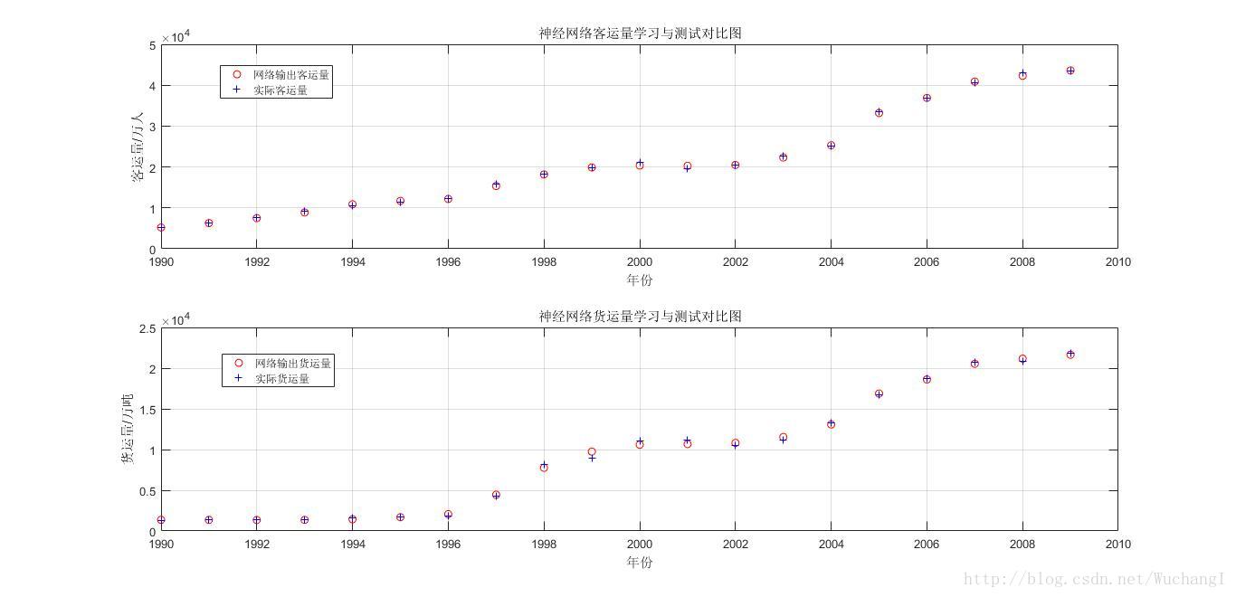
%绘制测试样本神经网络输出和实际样本输出的对比图(figure(1))--------------------------------------
t = 1990:2009;

%测试样本网络输出客运量
a1 = a(1,:); 
%测试样本网络输出货运量
a2 = a(2,:);

figure(1);
subplot(2, 1, 1); plot(t, a1, 'ro', t, passengerVolume, 'b+');
legend('网络输出客运量', '实际客运量');
xlabel('年份'); ylabel('客运量/万人');
title('神经网络客运量学习与测试对比图');
grid on;

subplot(2, 1, 2); plot(t, a2, 'ro', t, freightVolume, 'b+');
legend('网络输出货运量', '实际货运量');
xlabel('年份'); ylabel('货运量/万吨');
title('神经网络货运量学习与测试对比图');
grid on;

%使用训练好的神经网络对新输入数据进行预测

%新输入数据(2010年和2011年的相关数据)
newInput = [73.39 75.55; 3.9635 4.0975; 0.9880 1.0268]; 

%利用原始输入数据(训练集的输入数据)的归一化参数对新输入数据进行归一化
newInput = tramnmx(newInput, minp, maxp);

newHiddenOutput = logsig(W1 * newInput + repmat(B1, 1, numberOfForcastSample));
newOutput = W2 * newHiddenOutput + repmat(B2, 1, numberOfForcastSample);
newOutput = postmnmx(newOutput, mint, maxt);

disp('预测2010和2011年的公路客运量分别为(单位：万人)：');
newOutput(1,:)
disp('预测2010和2011年的公路货运量分别为(单位：万吨)：');
newOutput(2,:)

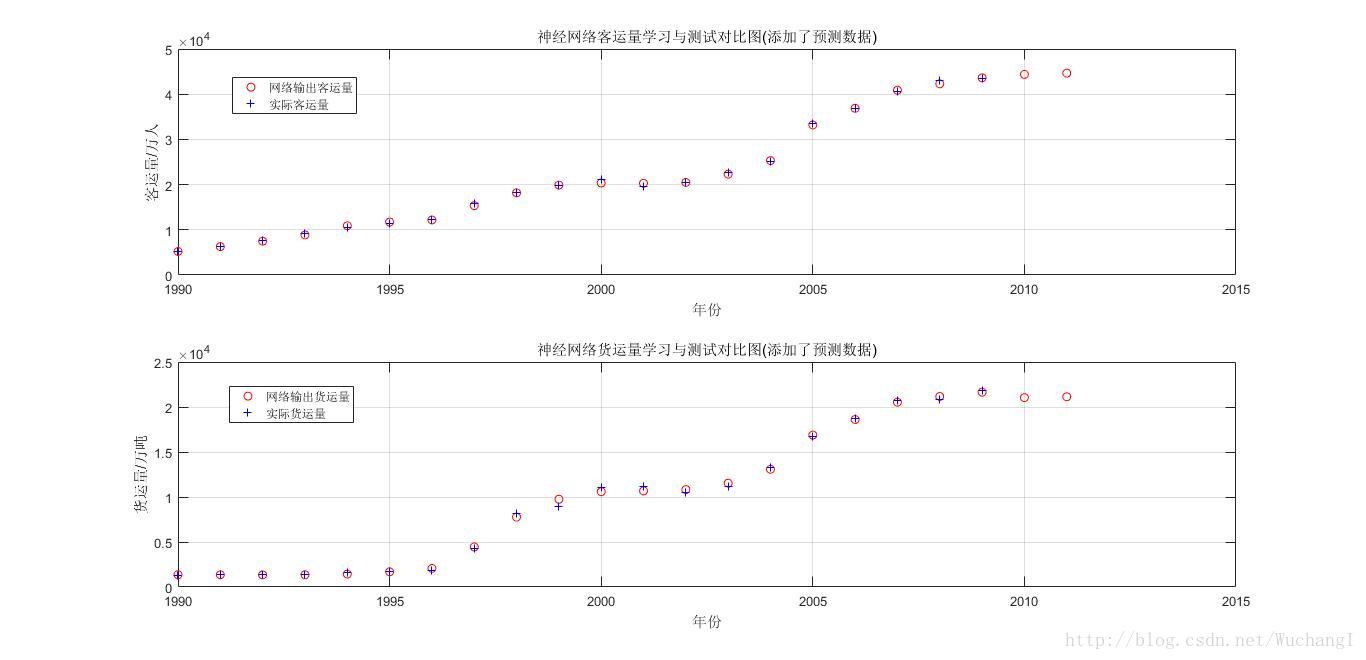
%在figure(1)的基础上绘制2010和2011年的预测情况-------------------------------------------------
figure(2);
t1 = 1990:2011;

subplot(2, 1, 1); plot(t1, [a1 newOutput(1,:)], 'ro', t, passengerVolume, 'b+');
legend('网络输出客运量', '实际客运量');
xlabel('年份'); ylabel('客运量/万人');
title('神经网络客运量学习与测试对比图(添加了预测数据)');
grid on;

subplot(2, 1, 2); plot(t1, [a2 newOutput(2,:)], 'ro', t, freightVolume, 'b+');
legend('网络输出货运量', '实际货运量');
xlabel('年份'); ylabel('货运量/万吨');
title('神经网络货运量学习与测试对比图(添加了预测数据)');
grid on;

%观察能量函数(误差平方和)在训练神经网络过程中的变化情况------------------------------------------
figure(3);

n = length(errorHistory);
t3 = 1:n;
plot(t3, errorHistory, 'r-');

%为了更加清楚地观察出能量函数值的变化情况，这里我只绘制前100次的训练情况
xlim([1 100]);
xlabel('训练过程');
ylabel('能量函数值');
title('能量函数(误差平方和)在训练神经网络过程中的变化图');
grid on;

4. 运行结果

预测2010和2011年的公路客运量分别为(单位：万人)：

ans =

1.0e+04 *

4.6188 4.6601

预测2010和2011年的公路货运量分别为(单位：万吨)：

ans =

1.0e+04 *

2.1521 2.1519

5. 绘制的图像

figure(1)

2. figure(2)

3. figure(3)

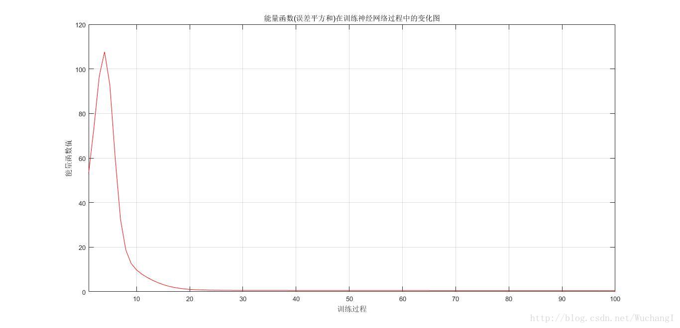
可以看出，使用BP网络中的负梯度下降原理之后，效果显著。

二. 使用MATLAB的神经网络工具箱简易实现BP网络

1. 问题

同<一>

2. 分析

同<一>

3. 工具箱中的相关函数(一些参考了MATLAB自带的英文手册)

mapminmax函数

功能：通过将原矩阵每行的最小值和最大值映射到[YMIN,YMAX]来得到规范化的矩阵。
算法：y = ( ymax - ymin ) * ( x - xmin ) / ( xmax - xmin ) + ymin

（注：当xmax与xmin相等时，则对原矩阵使用mapminmax函数仍得到原矩阵）

默认算法：

（默认情况下，mapminmax函数的YMIN和YMAX分别是-1和1）

y = 2 * ( x - xmin ) / ( xmax - xmin ) - 1

[Y,PS] = mapminmax(X)
- X：原矩阵
- Y：对矩阵X进行规范化得到的矩阵
- PS：存放关于原矩阵规范化过程中的相关映射数据的结构体
[Y,PS] = mapminmax(X,FP)
- X：原矩阵
- FP：含有字段FP.ymin和FP.ymax的结构体
- Y：对矩阵X进行规范化得到的矩阵（使用在FP的ymin和ymax规定下的算法）
- PS：存放关于原矩阵规范化过程中的相关映射数据的结构体
Y = mapminmax(‘apply’,X,PS)
- ’apply’：必写
- X：原矩阵
- PS：存放关于某个矩阵规范化过程中的相关映射数据的结构体
- Y：对矩阵X进行规范化得到的矩阵（使用PS中的规范化方式）
X = mapminmax(‘reverse’,Y,PS)
- ’reverse’：必写
- Y：某个矩阵
- PS：存放关于某个矩阵规范化过程中的相关映射数据的结构体
- X：将矩阵Y反规范化得到的矩阵（使用PS中的规范化方式，这里指将矩阵X转换为矩阵Y的规范化方式）

newff函数(新版本)

a. 功能：建立一个前馈反向传播（BP）网络。
b. net=newff（P,T,S）
- P: 输入数据矩阵。(RxQ1)，其中Q1代表R元的输入向量。其数据意义是矩阵P有Q1列，每一列都是一个样本，而每个样本有R个属性（特征）。一般矩阵P需要事先归一化好，即P的每一行都归一化到[0 1]或者[-1 1]。
- T：目标数据矩阵。(SNxQ2)，其中Q2代表SN元的目标向量。数据意义参考上面，矩阵T也是事先归一化好的。
- S：第i层的神经元个数。（新版本中可以省略输出层的神经元个数不写，因为输出层的神经元个数已经取决于T）
c. net = newff(P,T,S,TF,BTF,BLF,PF,IPF,OPF,DDF)（提供了可选择的参数）
- TF：相关层的传递函数，默认隐含层使用tansig函数，输出层使用purelin函数。
- BTF：BP神经网络学习训练函数，默认值为trainlm函数。
- BLF：权重学习函数，默认值为learngdm。
- PF：性能函数，默认值为mse。
- PF，OPF，DDF均为默认值即可。
d. 常用的传递函数:
- purelin：线性传递函数
- tansig：正切 S 型传递函数
- logsig：对数 S 型传递函数

(注意：隐含层和输出层函数的选择对BP神经网络预测精度有较大影响，一般隐含层节点传递函数选用tansig函数或logsig函数，输出层节点转移函数选用tansig函数或purelin函数。）

关于net.trainParam的常用属性

（假定已经定义了一个BP网络net）
* net.trainParam.show: 两次显示之间的训练次数
* net.trainParam.epochs: 最大训练次数
* net.trainParam.lr: 网络的学习速率
* net.trainParam.goal: 训练网络所要达到的目标误差
* net.trainParam.time: 最长训练时间（秒）

train函数

功能：训练一个神经网络
[NET2,TR] = train(NET1,X,T)（也可[NET2] = train(NET1,X,T) ）
- NET1：待训练的网络
- X: 输入数据矩阵（已归一化）
- T：目标数据矩阵（已归一化）
- NET2：训练得到的网络TR:存放有关训练过程的数据的结构体

sim函数

功能：模拟Simulink模型
SimOut = sim(‘MODEL’, PARAMETERS)
- （见名知意，不必再解释）

4. MATLAB实现代码

BP_toolbox_road.m

%准备好训练集

%人数(单位：万人)
numberOfPeople=[20.55 22.44 25.37 27.13 29.45 30.10 30.96 34.06 36.42 38.09 39.13 39.99 41.93 44.59 47.30 52.89 55.73 56.76 59.17 60.63];
%机动车数(单位：万辆)
numberOfAutomobile=[0.6 0.75 0.85 0.9 1.05 1.35 1.45 1.6 1.7 1.85 2.15 2.2 2.25 2.35 2.5 2.6 2.7 2.85 2.95 3.1];
%公路面积(单位：万平方公里)
roadArea=[0.09 0.11 0.11 0.14 0.20 0.23 0.23 0.32 0.32 0.34 0.36 0.36 0.38 0.49 0.56 0.59 0.59 0.67 0.69 0.79];
%公路客运量(单位：万人)
passengerVolume = [5126 6217 7730 9145 10460 11387 12353 15750 18304 19836 21024 19490 20433 22598 25107 33442 36836 40548 42927 43462];
%公路货运量(单位：万吨)
freightVolume = [1237 1379 1385 1399 1663 1714 1834 4322 8132 8936 11099 11203 10524 11115 13320 16762 18673 20724 20803 21804];

%输入数据矩阵
p = [numberOfPeople; numberOfAutomobile; roadArea];
%目标（输出）数据矩阵
t = [passengerVolume; freightVolume];

%对训练集中的输入数据矩阵和目标数据矩阵进行归一化处理
[pn, inputStr] = mapminmax(p);
[tn, outputStr] = mapminmax(t);

%建立BP神经网络
net = newff(pn, tn, [3 7 2], {'purelin', 'logsig', 'purelin'});

%每10轮回显示一次结果
net.trainParam.show = 10;

%最大训练次数
net.trainParam.epochs = 5000;

%网络的学习速率
net.trainParam.lr = 0.05;

%训练网络所要达到的目标误差
net.trainParam.goal = 0.65 * 10^(-3);

%网络误差如果连续6次迭代都没变化，则matlab会默认终止训练。为了让程序继续运行，用以下命令取消这条设置
net.divideFcn = '';

%开始训练网络
net = train(net, pn, tn);

%使用训练好的网络，基于训练集的数据对BP网络进行仿真得到网络输出结果
%(因为输入样本（训练集）容量较少，否则一般必须用新鲜数据进行仿真测试)
answer = sim(net, pn);

%反归一化
answer1 = mapminmax('reverse', answer, outputStr);

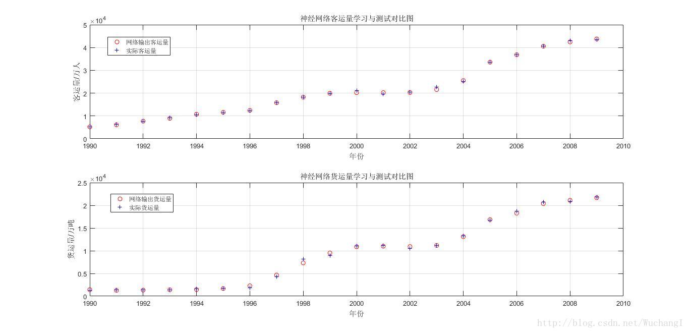
%绘制测试样本神经网络输出和实际样本输出的对比图(figure(1))-------------------------------------------
t = 1990:2009;

%测试样本网络输出客运量
a1 = answer1(1,:); 
%测试样本网络输出货运量
a2 = answer1(2,:);

figure(1);
subplot(2, 1, 1); plot(t, a1, 'ro', t, passengerVolume, 'b+');
legend('网络输出客运量', '实际客运量');
xlabel('年份'); ylabel('客运量/万人');
title('神经网络客运量学习与测试对比图');
grid on;

subplot(2, 1, 2); plot(t, a2, 'ro', t, freightVolume, 'b+');
legend('网络输出货运量', '实际货运量');
xlabel('年份'); ylabel('货运量/万吨');
title('神经网络货运量学习与测试对比图');
grid on;

%使用训练好的神经网络对新输入数据进行预测

%新输入数据(2010年和2011年的相关数据)
newInput = [73.39 75.55; 3.9635 4.0975; 0.9880 1.0268]; 

%利用原始输入数据(训练集的输入数据)的归一化参数对新输入数据进行归一化
newInput = mapminmax('apply', newInput, inputStr);

%进行仿真
newOutput = sim(net, newInput);

%反归一化
newOutput = mapminmax('reverse',newOutput, outputStr);

disp('预测2010和2011年的公路客运量分别为(单位：万人)：');
newOutput(1,:)
disp('预测2010和2011年的公路货运量分别为(单位：万吨)：');
newOutput(2,:)

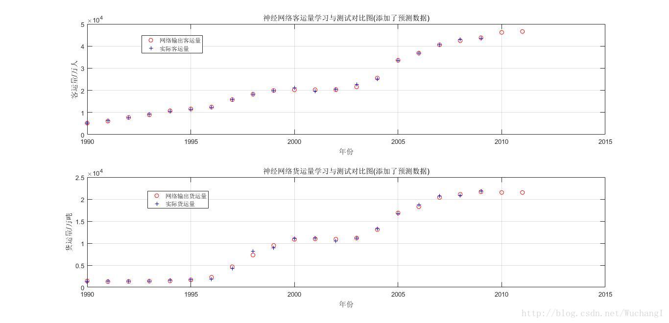
%在figure(1)的基础上绘制2010和2011年的预测情况-------------------------------------------------------
figure(2);
t1 = 1990:2011;

subplot(2, 1, 1); plot(t1, [a1 newOutput(1,:)], 'ro', t, passengerVolume, 'b+');
legend('网络输出客运量', '实际客运量');
xlabel('年份'); ylabel('客运量/万人');
title('神经网络客运量学习与测试对比图(添加了预测数据)');
grid on;

subplot(2, 1, 2); plot(t1, [a2 newOutput(2,:)], 'ro', t, freightVolume, 'b+');
legend('网络输出货运量', '实际货运量');
xlabel('年份'); ylabel('货运量/万吨');
title('神经网络货运量学习与测试对比图(添加了预测数据)');
grid on;

5. 运行结果

预测2010和2011年的公路客运量分别为(单位：万人)：

ans =

1.0e+04 *

4.4384 4.4656

预测2010和2011年的公路货运量分别为(单位：万吨)：

ans =

1.0e+04 *

2.1042 2.1139

6. 绘制的图像

figure(1)
figure(2)