R实战| 雷达图(Radar Chart)
雷达图(radar chart),又称蜘蛛网图(spider plot),是一种表现多维数据的强弱的图表。它将多个维度的数据量映射到坐标轴上,这些坐标轴起始于同一个圆心点,通常结束于圆周边缘,将同一组的点使用线连接起来就称为了雷达图。
本文以R包fmsb和 ggradar 为例介绍一下雷达图的绘制。
fmsb
install.packages("fmsb")
library(fmsb)
# 示例数据
exam_scores <- data.frame(
row.names = c("Student.1", "Student.2", "Student.3"),
Biology = c(7.9, 3.9, 9.4),
Physics = c(10, 20, 0),
Maths = c(3.7, 11.5, 2.5),
Sport = c(8.7, 20, 4),
English = c(7.9, 7.2, 12.4),
Geography = c(6.4, 10.5, 6.5),
Art = c(2.4, 0.2, 9.8),
Programming = c(0, 0, 20),
Music = c(20, 20, 20)
)
exam_scores> exam_scores
Biology Physics Maths Sport English Geography Art Programming Music
Student.1 7.9 10 3.7 8.7 7.9 6.4 2.4 0 20
Student.2 3.9 20 11.5 20.0 7.2 10.5 0.2 0 20
Student.3 9.4 0 2.5 4.0 12.4 6.5 9.8 20 20数据准备
数据要求:
第1行必须包含每个变量的最大值
第2行必须包含每个变量的最小值
列或变量的个数必须大于2
# 定义变量最大最小值
max_min <- data.frame(
  Biology = c(20, 0), Physics = c(20, 0), Maths = c(20, 0),
  Sport = c(20, 0), English = c(20, 0), Geography = c(20, 0),
  Art = c(20, 0), Programming = c(20, 0), Music = c(20, 0)
)
rownames(max_min) <- c("Max", "Min")

# 合并数据
df <- rbind(max_min, exam_scores)
df
> df
Biology Physics Maths Sport English Geography Art Programming Music
Max 20.0 20 20.0 20.0 20.0 20.0 20.0 20 20
Min 0.0 0 0.0 0.0 0.0 0.0 0.0 0 0
Student.1 7.9 10 3.7 8.7 7.9 6.4 2.4 0 20
Student.2 3.9 20 11.5 20.0 7.2 10.5 0.2 0 20
Student.3 9.4 0 2.5 4.0 12.4 6.5 9.8 20 20基础雷达图
#以student 1为例
library(fmsb)
student1_data <- df[c("Max", "Min", "Student.1"), ]
radarchart(student1_data)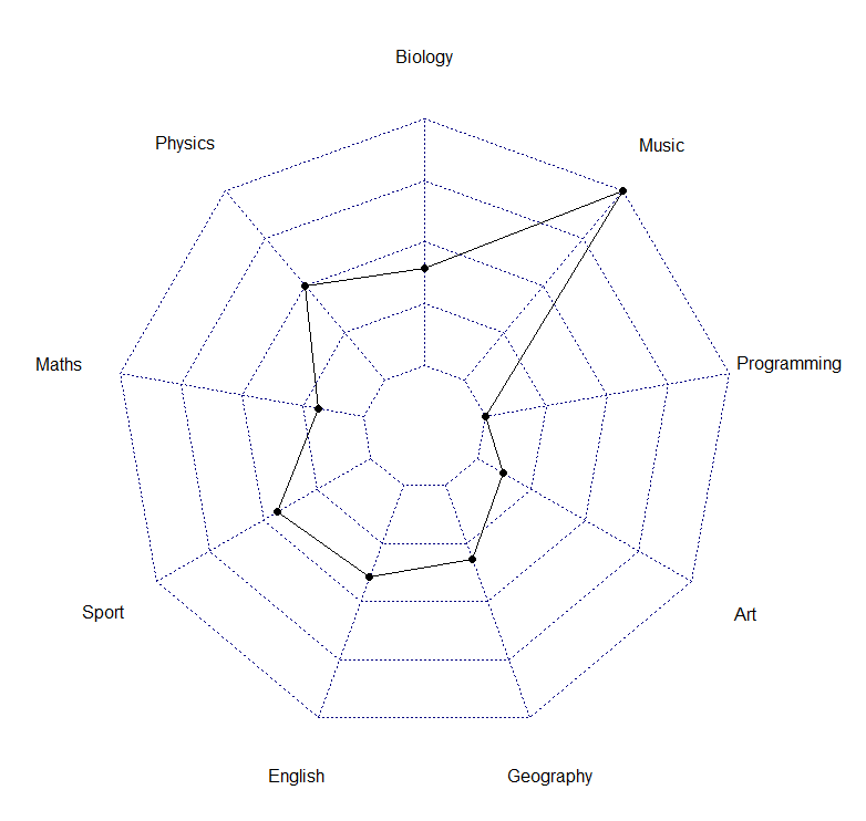
进阶雷达图
参数设置
Variable options
vlabels: 变量标签vlcex: 变量标签字体大小
Polygon options:
pcol: 线条颜色pfcol: 填充颜色plwd: 线条宽度plty: 线条类型. 使用数字1-6或者字符向量 (“solid”, “dashed”, “dotted”, “dotdash”, “longdash”, “twodash”).使用plty = 0orplty = “blank”,不显示线条.
Grid options:
cglcol:网格线颜色cglty: 网格线类型cglwd: 网格线宽度
Axis options:
axislabcol: 轴标签和数字的颜色。默认设置是“蓝色”。caxislabels: 字符向量,用作中心轴上的标签。
radarchart(
  student1_data, axistype = 1,
  # Customize the polygon
  pcol = "#00AFBB", pfcol = scales::alpha("#00AFBB", 0.5), plwd = 2, plty = 1,
  # Customize the grid
  cglcol = "grey", cglty = 1, cglwd = 0.8,
  # Customize the axis
  axislabcol = "grey",
  # Variable labels
  vlcex = 0.7, vlabels = colnames(student1_data),
  caxislabels = c(0, 5, 10, 15, 20))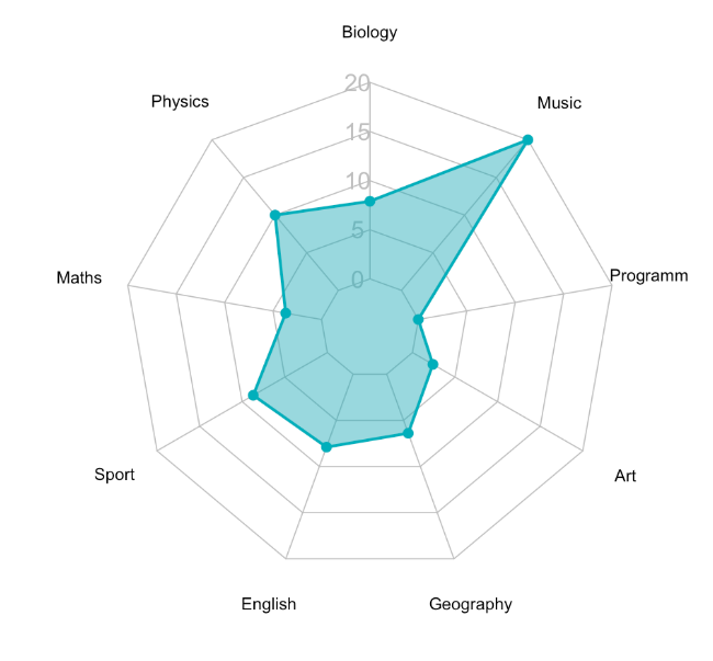
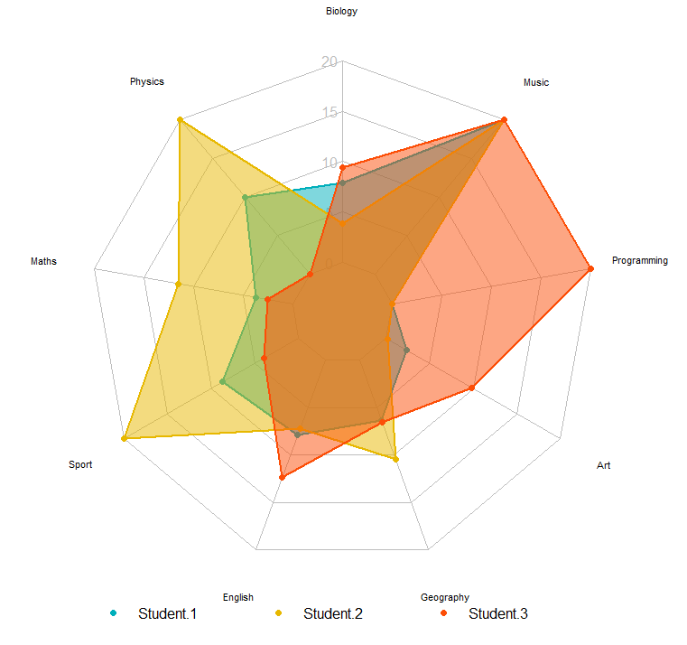
多组雷达图
radarchart(
  df, axistype = 1,
  # Customize the polygon
  pcol = c("#00AFBB", "#E7B800", "#FC4E07"), pfcol = scales::alpha(c("#00AFBB", "#E7B800", "#FC4E07"),0.5), plwd = 2, plty = 1,
  # Customize the grid
  cglcol = "grey", cglty = 1, cglwd = 0.8,
  # Customize the axis
  axislabcol = "grey",
  # Variable labels
  vlcex = 0.7, vlabels = colnames(student1_data),
  caxislabels = c(0, 5, 10, 15, 20))
# Add an horizontal legend
legend(
  x = "bottom", legend = rownames(df[-c(1,2),]), horiz = TRUE,
  bty = "n", pch = 20 , col = c("#00AFBB", "#E7B800", "#FC4E07"),
  text.col = "black", cex = 1, pt.cex = 1.5
)
ggradar
devtools::install_github("ricardo-bion/ggradar")
library("ggradar")
数据准备
library(tidyverse)
# 将行名改为分组列
df <- exam_scores %>% rownames_to_column("group")
df
> df
group Biology Physics Maths Sport English Geography Art Programming Music
1 Student.1 7.9 10 3.7 8.7 7.9 6.4 2.4 0 20
2 Student.2 3.9 20 11.5 20.0 7.2 10.5 0.2 0 20
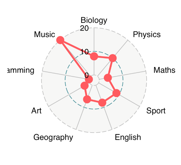
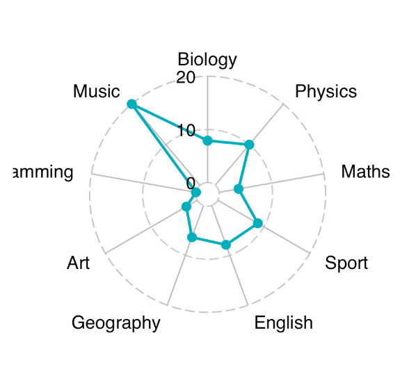
3 Student.3 9.4 0 2.5 4.0 12.4 6.5 9.8 20 20基础雷达图
ggradar(
  df[1, ],
  values.radar = c("0", "10", "20"),# 最小,平均和最大网格线显示的值
  grid.min = 0, # 绘制最小网格线的值
  grid.mid = 10, # 绘制平均网格线的值
  grid.max = 20 # 绘制最大网格线的值
)
进阶雷达图
ggradar(
  df[1, ],
  values.radar = c("0", "10", "20"),
  grid.min = 0, grid.mid = 10, grid.max = 20,
  # Polygons
  group.line.width = 1,
  group.point.size = 3,
  group.colours = "#00AFBB",
  # Background and grid lines
  background.circle.colour = "white",
  gridline.mid.colour = "grey"
)
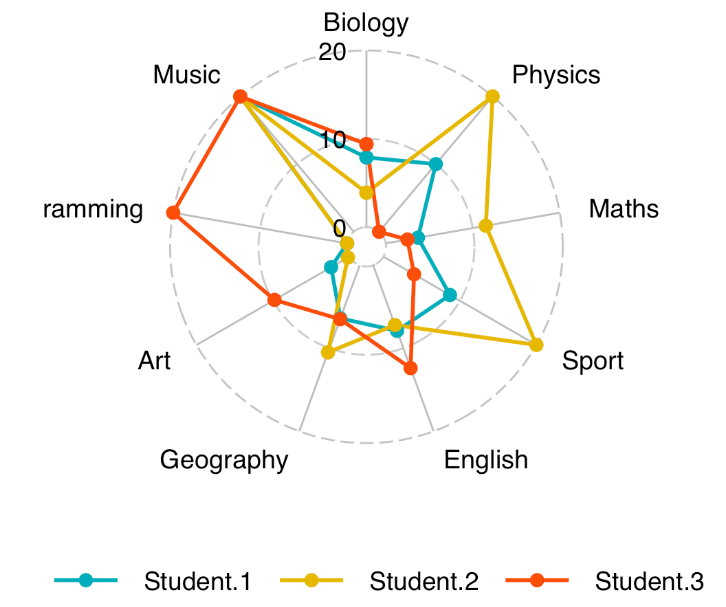
分组雷达图
ggradar(
  df,
  values.radar = c("0", "10", "20"),
  grid.min = 0, grid.mid = 10, grid.max = 20,
  # Polygons
  group.line.width = 1,
  group.point.size = 3,
  group.colours = c("#00AFBB", "#E7B800", "#FC4E07"),
  # Background and grid lines
  background.circle.colour = "white",
  gridline.mid.colour = "grey",
  legend.position = "bottom"
  )
Reference
https://www.datanovia.com/en/blog/beautiful-radar-chart-in-r-using-fmsb-and-ggplot-packages/
往期
- END -