该系列文章是讲解Python OpenCV图像处理知识,前期主要讲解图像入门、OpenCV基础用法,中期讲解图像处理的各种算法,包括图像锐化算子、图像增强技术、图像分割等,后期结合深度学习研究图像识别、图像分类应用。希望文章对您有所帮助,如果有不足之处,还请海涵~
上一篇文章分享了生成对抗网络GAN的基础知识,包括什么是GAN、常用算法(CGAN、DCGAN、infoGAN、WGAN)、发展历程、预备知识,并通过Keras搭建最简答的手写数字图片生成案例。这篇文章将详细讲解如何利用Keras构建AlexNet和CNN模型,实现自定义数据集的图像分类,并进行详细的对比。希望对您有所帮助!让我们开始吧,且看且珍惜。
第二阶段我们进入了Python图像识别,该部分主要以目标检测、图像识别以及深度学习相关图像分类为主,将会分享近50篇文章,感谢您一如至往的支持。作者也会继续加油的!

文章目录
同时,该部分知识均为作者查阅资料撰写总结,并且开设成了收费专栏,为小宝赚点奶粉钱,感谢您的抬爱。如果有问题随时私聊我,只望您能从这个系列中学到知识,一起加油。代码下载地址(如果喜欢记得star,一定喔):
图像识别:
- [Python图像识别] 四十五.对象检测案例入门及ImageAI基础用法
- [Python图像识别] 四十六.图像预处理之图像去雾详解(ACE算法和暗通道先验去雾算法)
- [Python图像识别] 四十七.Keras深度学习构建CNN识别阿拉伯手写文字图像
- [Python图像识别] 四十八.Pytorch构建Faster-RCNN模型实现小麦目标检测
- [Python图像识别] 四十九.图像生成之什么是生成对抗网络GAN?基础原理和代码普及
- [Python图像识别] 五十.Keras构建Alexnet和CNN实现自定义数据集分类详解
图像处理:
- [Python图像处理] 一.图像处理基础知识及OpenCV入门函数
- [Python图像处理] 二.OpenCV+Numpy库读取与修改像素
- [Python图像处理] 三.获取图像属性、兴趣ROI区域及通道处理
- [Python图像处理] 四.图像平滑之均值滤波、方框滤波、高斯滤波及中值滤波
- [Python图像处理] 五.图像融合、加法运算及图像类型转换
- [Python图像处理] 六.图像缩放、图像旋转、图像翻转与图像平移
- [Python图像处理] 七.图像阈值化处理及算法对比
- [Python图像处理] 八.图像腐蚀与图像膨胀
- [Python图像处理] 九.形态学之图像开运算、闭运算、梯度运算
- [Python图像处理] 十.形态学之图像顶帽运算和黑帽运算
- [Python图像处理] 十一.灰度直方图概念及OpenCV绘制直方图
- [Python图像处理] 十二.图像几何变换之图像仿射变换、图像透视变换和图像校正
- [Python图像处理] 十三.基于灰度三维图的图像顶帽运算和黑帽运算
- [Python图像处理] 十四.基于OpenCV和像素处理的图像灰度化处理
- [Python图像处理] 十五.图像的灰度线性变换
- [Python图像处理] 十六.图像的灰度非线性变换之对数变换、伽马变换
- [Python图像处理] 十七.图像锐化与边缘检测之Roberts算子、Prewitt算子、Sobel算子和Laplacian算子
- [Python图像处理] 十八.图像锐化与边缘检测之Scharr算子、Canny算子和LOG算子
- [Python图像处理] 十九.图像分割之基于K-Means聚类的区域分割
- [Python图像处理] 二十.图像量化处理和采样处理及局部马赛克特效
- [Python图像处理] 二十一.图像金字塔之图像向下取样和向上取样
- [Python图像处理] 二十二.Python图像傅里叶变换原理及实现
- [Python图像处理] 二十三.傅里叶变换之高通滤波和低通滤波
- [Python图像处理] 二十四.图像特效处理之毛玻璃、浮雕和油漆特效
- [Python图像处理] 二十五.图像特效处理之素描、怀旧、光照、流年以及滤镜特效
- [Python图像处理] 二十六.图像分类原理及基于KNN、朴素贝叶斯算法的图像分类案例
- [Python图像处理] 二十七.OpenGL入门及绘制基本图形(一)
- [Python图像处理] 二十八.OpenCV快速实现人脸检测及视频中的人脸
- [Python图像处理] 二十九.MoviePy视频编辑库实现抖音短视频剪切合并操作
- [Python图像处理] 三十.图像量化及采样处理万字详细总结(推荐)
- [Python图像处理] 三十一.图像点运算处理两万字详细总结(灰度化处理、阈值化处理)
- [Python图像处理] 三十二.傅里叶变换(图像去噪)与霍夫变换(特征识别)万字详细总结
- [Python图像处理] 三十三.图像各种特效处理及原理万字详解(毛玻璃、浮雕、素描、怀旧、流年、滤镜等)
- [Python图像处理] 三十四.数字图像处理基础与几何图形绘制万字详解(推荐)
- [Python图像处理] 三十五.OpenCV图像处理入门、算数逻辑运算与图像融合(推荐)
- [Python图像处理] 三十六.OpenCV图像几何变换万字详解(平移缩放旋转、镜像仿射透视)
- [Python图像处理] 三十七.OpenCV和Matplotlib绘制直方图万字详解(掩膜直方图、H-S直方图、黑夜白天判断)
- [Python图像处理] 三十八.OpenCV图像增强万字详解(直方图均衡化、局部直方图均衡化、自动色彩均衡化)
- [Python图像处理] 三十九.Python图像分类万字详解(贝叶斯图像分类、KNN图像分类、DNN图像分类)
- [Python图像处理] 四十.全网首发Python图像分割万字详解(阈值分割、边缘分割、纹理分割、分水岭算法、K-Means分割、漫水填充分割、区域定位)
- [Python图像处理] 四十一.Python图像平滑万字详解(均值滤波、方框滤波、高斯滤波、中值滤波、双边滤波)
- [Python图像处理] 四十二.Python图像锐化及边缘检测万字详解(Roberts、Prewitt、Sobel、Laplacian、Canny、LOG)
- [Python图像处理] 四十三.Python图像形态学处理万字详解(腐蚀膨胀、开闭运算、梯度顶帽黑帽运算)
- 万字长文告诉新手如何学习Python图像处理 (上篇完结 四十四)
一.图像分类概述
1.图像分类
图像分类(Image Classification)是对图像内容进行分类的问题,它利用计算机对图像进行定量分析,把图像或图像中的区域划分为若干个类别,以代替人的视觉判断。
图像分类的传统方法是特征描述及检测,这类传统方法可能对于一些简单的图像分类是有效的,但由于实际情况非常复杂,传统的分类方法不堪重负。现在,广泛使用机器学习和深度学习的方法来处理图像分类问题,其主要任务是给定一堆输入图片,将其指派到一个已知的混合类别中的某个标签。
在图1中,图像分类模型将获取单个图像,并将为4个标签{cat,dog,hat,mug}分配对应的概率{0.6, 0.3, 0.05, 0.05},其中0.6表示图像标签为猫的概率,其余类比。

如图1所示,该图像被表示为一个三维数组。在这个例子中,猫的图像宽度为248像素,高度为400像素,并具有红绿蓝三个颜色通道(通常称为RGB)。因此,图像由248×400×3个数字组成或总共297600个数字,每个数字是一个从0(黑色)到255(白色)的整数。图像分类的任务是将这接近30万个数字变成一个单一的标签,如“猫(cat)”。
那么,如何编写一个图像分类的算法呢?又怎么从众多图像中识别出猫呢?
这里所采取的方法和教育小孩看图识物类似,给出很多图像数据,让模型不断去学习每个类的特征。在训练之前,首先需要对训练集的图像进行分类标注,如图2所示,包括cat、dog、mug和hat四类。在实际工程中,可能有成千上万类别的物体,每个类别都会有上百万张图像。

图像分类是输入一堆图像的像素值数组,然后给它分配一个分类标签,通过训练学习来建立算法模型,接着使用该模型进行图像分类预测,具体流程如下:
- 输入:输入包含N个图像的集合,每个图像的标签是K种分类标签中的一种,这个集合称为训练集;
- 学习:第二步任务是使用训练集来学习每个类的特征,构建训练分类器或者分类模型;
- 评价:通过分类器来预测新输入图像的分类标签,并以此来评价分类器的质量。通过分类器预测的标签和图像真正的分类标签对比,从而评价分类算法的好坏。如果分类器预测的分类标签和图像真正的分类标签一致,表示预测正确,否则预测错误。
2.数据集
实验所采用的数据集为Sort_1000pics数据集,该数据集包含了1000张图片,总共分为10大类,分别是人(第0类)、沙滩(第1类)、建筑(第2类)、大卡车(第3类)、恐龙(第4类)、大象(第5类)、花朵(第6类)、马(第7类)、山峰(第8类)和食品(第9类),每类100张。如图11所示。

接着将所有各类图像按照对应的类标划分至“0”至“9”命名的文件夹中,如图12所示,每个文件夹中均包含了100张图像,对应同一类别。

比如,文件夹名称为“6”中包含了100张花的图像,如图13所示。

二.基于NB的图像分类
1.朴素贝叶斯分类算法
朴素贝叶斯分类(Naive Bayes Classifier)发源于古典数学理论,利用Bayes定理来预测一个未知类别的样本属于各个类别的可能性,选择其中可能性最大的一个类别作为该样本的最终类别。在朴素贝叶斯分类模型中,它将为每一个类别的特征向量建立服从正态分布的函数,给定训练数据,算法将会估计每一个类别的向量均值和方差矩阵,然后根据这些进行预测。

朴素贝叶斯分类模型的正式定义如下:

该算法的特点为:如果没有很多数据,该模型会比很多复杂的模型获得更好的性能,因为复杂的模型用了太多假设,以致产生欠拟合。
2.代码实现
下面是调用朴素贝叶斯算法进行图像分类的完整代码,调用sklearn.naive_bayes中的BernoulliNB()函数进行实验。它将1000张图像按照训练集为70%,测试集为30%的比例随机划分,再获取每张图像的像素直方图,根据像素的特征分布情况进行图像分类分析。
注意:机器学习代码是统计灰度直方图,再进行的图像分类预测。而后续深度学习采用读取图像像素,对其进行分类的。
# -*- coding: utf-8 -*-
"""
Created on Fri Apr  8 22:02:29 2022
@author: xiuzhang
"""
import os
import cv2
import numpy as np
from sklearn.model_selection import train_test_split
from sklearn.metrics import confusion_matrix, classification_report

#----------------------------------------------------------------------------------
# 第一步 切分训练集和测试集
#----------------------------------------------------------------------------------
X = [] #定义图像名称
Y = [] #定义图像分类类标
Z = [] #定义图像像素

for i in range(0, 10):
    #遍历文件夹,读取图片
    for f in os.listdir("data/%s" % i):
        #获取图像名称
        X.append("data//" +str(i) + "//" + str(f))
        #获取图像类标即为文件夹名称
        Y.append(i)
X = np.array(X)
Y = np.array(Y)

#随机率为100% 选取其中的30%作为测试集
X_train, X_test, y_train, y_test = train_test_split(X, Y,
test_size=0.3, random_state=1)
print(len(X_train), len(X_test), len(y_train), len(y_test))

#----------------------------------------------------------------------------------
# 第二步 图像读取及转换为像素直方图
#----------------------------------------------------------------------------------
#训练集
XX_train = []
for i in X_train:
    #读取图像
    image = cv2.imread(i)
    #图像像素大小一致
    img = cv2.resize(image, (256,256),
                     interpolation=cv2.INTER_CUBIC)
    #计算图像直方图并存储至X数组
    hist = cv2.calcHist([img], [0,1], None,
                            [256,256], [0.0,255.0,0.0,255.0])
    XX_train.append(((hist/255).flatten()))

#测试集
XX_test = []
for i in X_test:
    #读取图像
    image = cv2.imread(i)
    #图像像素大小一致
    img = cv2.resize(image, (256,256),
                     interpolation=cv2.INTER_CUBIC)
    #计算图像直方图并存储至X数组
    hist = cv2.calcHist([img], [0,1], None,
                            [256,256], [0.0,255.0,0.0,255.0])
    XX_test.append(((hist/255).flatten()))

#----------------------------------------------------------------------------------
# 第三步 基于朴素贝叶斯的图像分类处理
#----------------------------------------------------------------------------------
from sklearn.naive_bayes import BernoulliNB
clf = BernoulliNB().fit(XX_train, y_train)
predictions_labels = clf.predict(XX_test)
print('预测结果:')
print(predictions_labels)
print('算法评价:')
print(classification_report(y_test, predictions_labels,digits=4))

#输出前10张图片及预测结果
k = 0
while k<10:
    #读取图像
    print(X_test[k])
    image = cv2.imread(X_test[k])
    print(predictions_labels[k])
    #显示图像
    cv2.imshow("img", image)
    cv2.waitKey(0)
    cv2.destroyAllWindows()
    k = k + 1
3.结果评估
输出结果如下所示:
700 300 700 300
预测结果:
[7 8 4 3 2 9 2 4 3 9 4 9 0 3 0 8 8 5 7 4 9 4 2 5 4 1 2 7 2 3 9 7 7 4 8 2 2
 5 7 4 1 6 9 2 9 2 5 2 4 3 2 0 6 0 1 4 8 6 4 9 3 2 3 7 8 5 4 8 0 2 2 8 2 9
 4 2 1 8 3 5 2 7 7 7 9 9 4 8 2 5 6 1 5 9 4 8 5 8 2 8 3 2 9 8 4 5 2 5 4 9 4
 9 9 0 1 0 7 4 1 7 2 3 9 1 4 6 7 7 4 9 9 2 6 0 9 2 7 8 8 7 2 8 9 5 6 7 7 9
 5 2 3 9 1 0 3 5 7 8 0 2 8 2 1 6 5 4 2 5 7 8 2 2 8 4 5 2 1 9 8 9 2 0 7 6 2
 8 2 4 5 0 6 1 2 1 9 4 5 5 6 2 3 7 9 0 5 7 0 0 3 4 7 3 8 4 6 8 3 1 9 9 8 8
 8 9 5 7 0 7 9 8 2 3 8 4 5 9 0 7 2 0 8 5 3 4 4 8 8 4 8 7 2 0 4 7 0 6 9 8 8
 7 8 8 1 0 7 4 3 4 4 8 4 0 8 5 9 7 8 2 6 0 7 8 3 7 5 2 8 1 4 9 6 5 5 1 8 4
 4 0 2 3]
算法评价:
              precision    recall  f1-score   support

           0     0.5000    0.3871    0.4364        31
           1     0.6471    0.3548    0.4583        31
           2     0.4651    0.7692    0.5797        26
           3     0.8095    0.5862    0.6800        29
           4     0.7692    0.9375    0.8451        32
           5     0.5714    0.4706    0.5161        34
           6     0.8667    0.4333    0.5778        30
           7     0.5588    0.7308    0.6333        26
           8     0.4773    0.6774    0.5600        31
           9     0.6571    0.7667    0.7077        30

    accuracy                         0.6067       300
   macro avg     0.6322    0.6114    0.5994       300
weighted avg     0.6340    0.6067    0.5984       300
三.基于CNN的图像分类
1.卷积神经网络概念
卷积神经网络的英文是Convolutional Neural Network,简称CNN。它通常应用于图像识别和语音识等领域,并能给出更优秀的结果,也可以应用于视频分析、机器翻译、自然语言处理、药物发现等领域。著名的阿尔法狗让计算机看懂围棋就是基于卷积神经网络的。
神经网络是由很多神经层组成,每一层神经层中存在很多神经元,这些神经元是识别事物的关键,当输入是图片时,其实就是一堆数字。
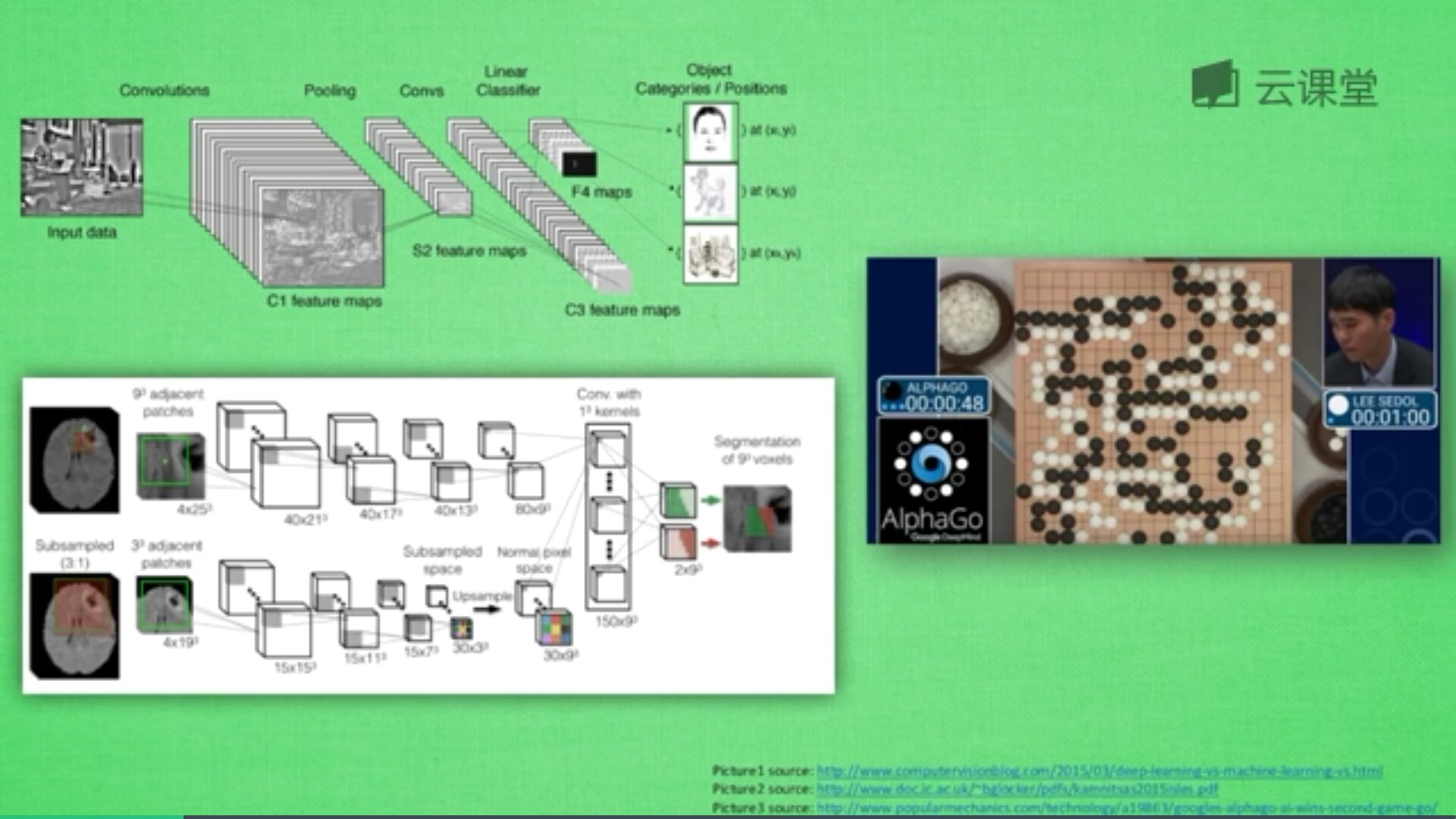
首先,卷积是什么意思呢?
卷积是指不在对每个像素做处理,而是对图片区域进行处理,这种做法加强了图片的连续性,看到的是一个图形而不是一个点,也加深了神经网络对图片的理解。
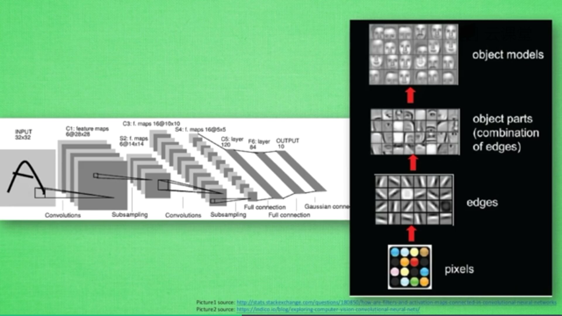
卷积神经网络批量过滤器,持续不断在图片上滚动搜集信息,每一次搜索都是一小块信息,整理这一小块信息之后得到边缘信息。比如第一次得出眼睛鼻子轮廓等,再经过一次过滤,将脸部信息总结出来,再将这些信息放到全神经网络中进行训练,反复扫描最终得出的分类结果。如下图所示,猫的一张照片需要转换为数学的形式,这里采用长宽高存储,其中黑白照片的高度为1,彩色照片的高度为3(RGB)。

过滤器搜集这些信息,将得到一个更小的图片,再经过压缩增高信息嵌入到普通神经层上,最终得到分类的结果,这个过程即是卷积。Convnets是一种在空间上共享参数的神经网络,如下图所示,它将一张RGB图片进行压缩增高,得到一个很长的结果。

一个卷积网络是组成深度网络的基础,我们将使用数层卷积而不是数层的矩阵相乘。如上图所示,让它形成金字塔形状,金字塔底是一个非常大而浅的图片,仅包括红绿蓝,通过卷积操作逐渐挤压空间的维度,同时不断增加深度,使深度信息基本上可以表示出复杂的语义。同时,你可以在金字塔的顶端实现一个分类器,所有空间信息都被压缩成一个标识,只有把图片映射到不同类的信息保留,这就是CNN的总体思想。
2.代码实现
CNN代码如下所示:
# -*- coding: utf-8 -*-
"""
Created on Fri Apr  8 22:01:24 2022
@author: xiuzhang
"""
import os
import cv2
import numpy as np
import matplotlib.pyplot as plt
from sklearn.model_selection import train_test_split
from sklearn.metrics import confusion_matrix, classification_report
from keras.utils import np_utils
from keras.models import Sequential
from keras.layers import Dense, Activation, BatchNormalization, Dropout
from keras.layers import Conv2D, MaxPooling2D, GlobalAveragePooling2D
from keras.callbacks import ModelCheckpoint
from keras.callbacks import EarlyStopping

#-----------------------------------------------------------------------
# 第一步 切分训练集和测试集
#-----------------------------------------------------------------------
X = [] #定义图像名称
Y = [] #定义图像分类类标
Z = [] #定义图像像素

for i in range(0, 10):
    #遍历文件夹,读取图片
    for f in os.listdir("data/%s" % i):
        #获取图像名称
        X.append("data//" +str(i) + "//" + str(f))
        #获取图像类标即为文件夹名称
        Y.append(i)
X = np.array(X)
Y = np.array(Y)

#随机率为100% 选取其中的30%作为测试集
X_train, X_test, y_train, y_test = train_test_split(X, Y,
test_size=0.3, random_state=1)
print(len(X_train), len(X_test), len(y_train), len(y_test))

#------------------------------------------------------------------------
# 第二步 图像读取及转换为像素直方图
#------------------------------------------------------------------------
#训练集
XX_train = []
for i in X_train:
    image = cv2.imread(i)
    img = cv2.resize(image,(128,128),interpolation=cv2.INTER_CUBIC)
    res = img.astype('float32')/255.0
    #print(img)
    #print(img.shape)  #(256, 256, 3)
    #print(res)
    XX_train.append(res)
#测试集
XX_test = []
for i in X_test:
    image = cv2.imread(i)
    img = cv2.resize(image,(128,128),interpolation=cv2.INTER_CUBIC)
    res = img.astype('float32')/255.0
    XX_test.append(res)

train_images_scaled =  np.array(XX_train)
test_images_scaled =  np.array(XX_test)
for n in train_images_scaled:
    print(n)
    break
print(type(train_images_scaled))
print(train_images_scaled.shape,test_images_scaled.shape)
# <class 'numpy.ndarray'>
# (700, 256, 256, 3) (300, 256, 256, 3)

#将类向量转化为类矩阵 [0 0 0 0 0 1 0 0 0 0]
train_labels_encoded = np_utils.to_categorical(y_train, num_classes=10)
test_labels_encoded = np_utils.to_categorical(y_test, num_classes=10)
print(train_labels_encoded.shape, test_labels_encoded.shape)

#---------------------------------------------------------------------
# 第三步 CNN模型设计
#---------------------------------------------------------------------
#定义模型
def create_model(optimizer='adam', kernel_initializer='he_normal', activation='relu'):
    model = Sequential()
    model.add(Conv2D(filters=128,
                     kernel_size=16,
                     padding='same',
                     input_shape=(128, 128, 3),
                     activation=activation))
    model.add(MaxPooling2D(pool_size=16))
    model.add(Dropout(0.3))
    model.add(GlobalAveragePooling2D())
    model.add(Dense(10, activation='softmax'))
    model.compile(loss='categorical_crossentropy',
                  metrics=['accuracy'],
                  optimizer=optimizer)
    return model

#创建模型
model = create_model(optimizer='Adam',
                     kernel_initializer='uniform',
                     activation='relu')
model.summary()

#----------------------------------------------------------------
# 第四步 模型绘制
#----------------------------------------------------------------
from keras.utils.vis_utils import plot_model
from IPython.display import Image as IPythonImage
plot_model(model, to_file="model.png", show_shapes=True)
display(IPythonImage('model.png'))

#绘制图形
def plot_loss_accuracy(history):
    # Loss
    plt.figure(figsize=[8,6])
    plt.plot(history.history['loss'],'r',linewidth=3.0)
    plt.plot(history.history['val_loss'],'b',linewidth=3.0)
    plt.legend(['Training loss', 'Validation Loss'],fontsize=18)
    plt.xlabel('Epochs ',fontsize=16)
    plt.ylabel('Loss',fontsize=16)
    plt.title('Loss Curves',fontsize=16)

    # Accuracy
    plt.figure(figsize=[8,6])
    plt.plot(history.history['accuracy'],'r',linewidth=3.0)
    plt.plot(history.history['val_accuracy'],'b',linewidth=3.0)
    plt.legend(['Training Accuracy', 'Validation Accuracy'],fontsize=18)
    plt.xlabel('Epochs ',fontsize=16)
    plt.ylabel('Accuracy',fontsize=16)
    plt.title('Accuracy Curves',fontsize=16)

#混淆矩阵
def get_predicted_classes(model, data, labels=None):
    image_predictions = model.predict(data)
    predicted_classes = np.argmax(image_predictions, axis=1)
    true_classes = np.argmax(labels, axis=1)
    return predicted_classes, true_classes, image_predictions

def get_classification_report(y_true, y_pred):
    print(classification_report(y_true, y_pred, digits=4)) #小数点4位

checkpointer = ModelCheckpoint(filepath='weights-cnn.hdf5',
                               verbose=1,
                               save_best_only=True)
#EarlyStopping(monitor='val_loss',min_delta=0.0005)

#----------------------------------------------------------------
# 第五步 模型训练测试
#----------------------------------------------------------------
flag = "test"
if flag=="train":
    history = model.fit(train_images_scaled,
                        train_labels_encoded,
                        validation_data=(test_images_scaled,test_labels_encoded),
                        epochs=15,
                        batch_size=64,
                        callbacks=[checkpointer])
    print(history)
    plot_loss_accuracy(history)
else:
    #加载具有最佳验证损失的模型
    model.load_weights('weights-cnn.hdf5')
    metrics = model.evaluate(test_images_scaled,
                             test_labels_encoded,
                             verbose=1)
    print("Test Accuracy: {}".format(metrics[1]))
    print("Test Loss: {}".format(metrics[0]))

    y_pred, y_true, image_predictions = get_predicted_classes(model,
                                                              test_images_scaled,
                                                              test_labels_encoded)
    get_classification_report(y_true, y_pred)
3.结果评估
生成的模型如下所示:

评估结果如下:
700 300 700 300
<class 'numpy.ndarray'>
(700, 128, 128, 3) (300, 128, 128, 3)
(700, 10) (300, 10)
Model: "sequential_7"
_________________________________________________________________
Layer (type)                 Output Shape              Param #
=================================================================
conv2d_7 (Conv2D)            (None, 128, 128, 128)     98432
_________________________________________________________________
max_pooling2d_7 (MaxPooling2 (None, 8, 8, 128)         0
_________________________________________________________________
dropout_7 (Dropout)          (None, 8, 8, 128)         0
_________________________________________________________________
global_average_pooling2d_7 ( (None, 128)               0
_________________________________________________________________
dense_7 (Dense)              (None, 10)                1290
=================================================================
Total params: 99,722
Trainable params: 99,722
Non-trainable params: 0
_________________________________________________________________

10/10 [==============================] - 7s 632ms/step - loss: 1.3755 - accuracy: 0.5533
Test Accuracy: 0.5533333420753479
Test Loss: 1.3755393028259277
              precision    recall  f1-score   support

           0     0.4737    0.5806    0.5217        31
           1     0.4783    0.3548    0.4074        31
           2     0.5882    0.3846    0.4651        26
           3     1.0000    0.6207    0.7660        29
           4     0.5167    0.9688    0.6739        32
           5     0.3556    0.4706    0.4051        34
           6     0.6000    0.6000    0.6000        30
           7     0.8462    0.8462    0.8462        26
           8     0.4091    0.2903    0.3396        31
           9     0.6190    0.4333    0.5098        30

    accuracy                         0.5533       300
   macro avg     0.5887    0.5550    0.5535       300
weighted avg     0.5789    0.5533    0.5476       300
四.基于AlexNet的图像分类
1.AlexNet模型
从严格意义上讲,卷积网络模型的开山之作应该是LeNet,由深度学习三巨头之一的杨立坤(Yann LeCun)在1998年提出来的,用来解决手写数字识别问题,但是由于年代久远,而且由于当时算力有限,深度学习一直没有得到发展,直到2012年AlexNet分类网络横空出世,首次证明学习到的特征,可以远远超过人工设计的特征,一举颠覆了计算机视觉研究方向,在ImageNet大赛上一举夺魁,遥遥领先传统分类方法!
—— 知乎 大橙子老师
推荐大家阅读三位老师的博客:
- https://d2l.ai/chapter_convolutional-modern/alexnet.html
- 【图像分类】 一文读懂AlexNet
- 妈妈再不担心系列之图像分类——AlexNet(详细代码)

AlexNet模型如下图所示,推荐大家阅读论文原文。结构包括:
- 8层网络:5个卷积和3个全连接
- AlexNet第一层中的卷积核shape为11x11,第二层的卷积核形状缩小到5x5,之后全部采用3x3的卷积核
- 所有的池化层窗口大小为3x3,步长为2,最大池化
- 采用Relu激活函数,代替sigmoid,梯度计算更简单,模型更容易训练
- 采用Dropout来控制模型复杂度,防止过拟合
- 采用大量图像增强技术,比如翻转、裁剪和颜色变化,扩大数据集,防止过拟合

Keras核心代码如下:

2.代码实现
# -*- coding: utf-8 -*-
"""
Created on Fri Apr  8 22:01:24 2022
@author: xiuzhang
"""
import os
import cv2
import numpy as np
import matplotlib.pyplot as plt
from sklearn.model_selection import train_test_split
from sklearn.metrics import confusion_matrix, classification_report
from keras.utils import np_utils
from keras.models import Sequential
from keras.layers import Dense, Activation, BatchNormalization, Dropout, Flatten
from keras.layers import Conv2D, MaxPooling2D, GlobalAveragePooling2D
from keras.callbacks import ModelCheckpoint

#GPU加速
import os
import tensorflow as tf
os.environ["CUDA_DEVICES_ORDER"] = "PCI_BUS_IS"
os.environ["CUDA_VISIBLE_DEVICES"] = "0"

#指定了每个GPU进程中使用显存的上限,0.9表示可以使用GPU 90%的资源进行训练
gpu_options = tf.GPUOptions(per_process_gpu_memory_fraction=0.8)
sess = tf.Session(config=tf.ConfigProto(gpu_options=gpu_options))

#-----------------------------------------------------------------------
# 第一步 切分训练集和测试集
#-----------------------------------------------------------------------
X = [] #定义图像名称
Y = [] #定义图像分类类标
Z = [] #定义图像像素

for i in range(0, 10):
    #遍历文件夹,读取图片
    for f in os.listdir("data/%s" % i):
        #获取图像名称
        X.append("data//" +str(i) + "//" + str(f))
        #获取图像类标即为文件夹名称
        Y.append(i)
X = np.array(X)
Y = np.array(Y)

#随机率为100% 选取其中的30%作为测试集
X_train, X_test, y_train, y_test = train_test_split(X, Y,
                                                    test_size=0.3,
                                                    random_state=1)
print(len(X_train), len(X_test), len(y_train), len(y_test))

#------------------------------------------------------------------------
# 第二步 图像读取及转换为像素直方图
#------------------------------------------------------------------------
#训练集
XX_train = []
for i in X_train:
    image = cv2.imread(i)
    img = cv2.resize(image,(224,224),interpolation=cv2.INTER_CUBIC)
    res = img.astype('float32')/255
    #print(img)
    #print(img.shape)  #(256, 256, 3)
    #print(res)
    XX_train.append(res)

#测试集
XX_test = []
for i in X_test:
    image = cv2.imread(i)
    img = cv2.resize(image,(224,224),interpolation=cv2.INTER_CUBIC)
    res = img.astype('float32')/255
    XX_test.append(res)

train_images_scaled =  np.array(XX_train)
test_images_scaled =  np.array(XX_test)
print(type(train_images_scaled))
print(train_images_scaled.shape,test_images_scaled.shape)
# <class 'numpy.ndarray'>
# (700, 256, 256, 3) (300, 256, 256, 3)

#将类向量转化为类矩阵 [0 0 0 0 0 1 0 0 0 0]
train_labels_encoded = np_utils.to_categorical(y_train, num_classes=10)
test_labels_encoded = np_utils.to_categorical(y_test, num_classes=10)
print(train_labels_encoded.shape, test_labels_encoded.shape)

#---------------------------------------------------------------------
# 第三步 AlexNet模型设计
#---------------------------------------------------------------------
#定义模型
def create_model(optimizer='adam', kernel_initializer='he_normal', activation='relu'):
    #第一层卷积
    #卷积核数量96 尺寸11*11 步长4 激活函数relu
    #最大池化 尺寸3*3,步长2
    model = Sequential()
    model.add(Conv2D(filters=96,
                     kernel_size=11,
                     strides=4,
                     input_shape=(224, 224, 3),
                     activation=activation))
    model.add(MaxPooling2D(pool_size=3, strides=2))

    #第二层卷积
    #卷积核数量256 尺寸5*5 激活函数relu same卷积
    #最大池化 尺寸3*3,步长2
    model.add(Conv2D(filters=256,
                     kernel_size=5,
                     padding='same',
                     activation=activation))
    model.add(MaxPooling2D(pool_size=3, strides=2))

    #第三层卷积
    #卷积核数量384 尺寸3 激活函数relu same卷积
    model.add(Conv2D(filters=384,
                     kernel_size=3,
                     padding='same',
                     activation=activation))

    #第四层卷积
    #卷积核数量384 尺寸3 激活函数relu same卷积
    model.add(Conv2D(filters=384,
                     kernel_size=3,
                     padding='same',
                     activation=activation))

    #第五层卷积
    #卷积核数量256 尺寸3 激活函数relu same卷积
    #最大池化 尺寸3*3,步长2
    model.add(Conv2D(filters=256,
                     kernel_size=3,
                     padding='same',
                     activation=activation))
    model.add(MaxPooling2D(pool_size=3, strides=2))

    #展平特征图
    model.add(Flatten())

    #第一个全连接 4096神经元 relu
    model.add(Dense(4096, activation='relu'))
    model.add(Dropout(0.5))

    #第二个全连接 4096神经元 relu
    model.add(Dense(4096, activation='relu'))
    model.add(Dropout(0.5))

    #第二个全连接 输出10类结果
    model.add(Dense(10, activation='softmax'))

    #损失函数定义
    model.compile(loss='categorical_crossentropy',
                  metrics=['accuracy'],
                  optimizer=optimizer)
    return model

#创建模型
model = create_model(optimizer='Adam',
                     kernel_initializer='uniform',
                     activation='relu')
model.summary()

#----------------------------------------------------------------
# 第四步 模型绘制
#----------------------------------------------------------------
from keras.utils.vis_utils import plot_model
from IPython.display import Image as IPythonImage
plot_model(model, to_file="AlexNet-model.png", show_shapes=True)
display(IPythonImage('AlexNet-model.png'))

#绘制图形
def plot_loss_accuracy(history):
    # Loss
    plt.figure(figsize=[8,6])
    plt.plot(history.history['loss'],'r',linewidth=3.0)
    plt.plot(history.history['val_loss'],'b',linewidth=3.0)
    plt.legend(['Training loss', 'Validation Loss'],fontsize=18)
    plt.xlabel('Epochs ',fontsize=16)
    plt.ylabel('Loss',fontsize=16)
    plt.title('Loss Curves',fontsize=16)

    # Accuracy
    plt.figure(figsize=[8,6])
    plt.plot(history.history['accuracy'],'r',linewidth=3.0)
    plt.plot(history.history['val_accuracy'],'b',linewidth=3.0)
    plt.legend(['Training Accuracy', 'Validation Accuracy'],fontsize=18)
    plt.xlabel('Epochs ',fontsize=16)
    plt.ylabel('Accuracy',fontsize=16)
    plt.title('Accuracy Curves',fontsize=16)

#混淆矩阵
def get_predicted_classes(model, data, labels=None):
    image_predictions = model.predict(data)
    predicted_classes = np.argmax(image_predictions, axis=1)
    true_classes = np.argmax(labels, axis=1)
    return predicted_classes, true_classes, image_predictions

def get_classification_report(y_true, y_pred):
    print(classification_report(y_true, y_pred, digits=4)) #小数点4位

checkpointer = ModelCheckpoint(filepath='weights-AlexNet.hdf5',
                               verbose=1,
                               save_best_only=True)

#----------------------------------------------------------------
# 第五步 模型训练测试
#----------------------------------------------------------------
flag = "train"
if flag=="train":
    history = model.fit(train_images_scaled,
                        train_labels_encoded,
                        validation_data=(test_images_scaled,test_labels_encoded),
                        epochs=15,
                        batch_size=20,
                        verbose=1,
                        callbacks=[checkpointer])
    print(history)
    plot_loss_accuracy(history)
else:
    #加载具有最佳验证损失的模型
    model.load_weights('weights-AlexNet.hdf5')
    metrics = model.evaluate(test_images_scaled,
                             test_labels_encoded,
                             verbose=1)
    print("Test Accuracy: {}".format(metrics[1]))
    print("Test Loss: {}".format(metrics[0]))

    y_pred, y_true, image_predictions = get_predicted_classes(model,
                                                              test_images_scaled,
                                                              test_labels_encoded)
    get_classification_report(y_true, y_pred)
3.结果评估
输出结果如下图所示:
700 300 700 300
<class 'numpy.ndarray'>
(700, 224, 224, 3) (300, 224, 224, 3)
(700, 10) (300, 10)
Model: "sequential_12"
_________________________________________________________________
Layer (type)                 Output Shape              Param #
=================================================================
conv2d_28 (Conv2D)           (None, 54, 54, 96)        34944
_________________________________________________________________
max_pooling2d_20 (MaxPooling (None, 26, 26, 96)        0
_________________________________________________________________
conv2d_29 (Conv2D)           (None, 26, 26, 256)       614656
_________________________________________________________________
max_pooling2d_21 (MaxPooling (None, 12, 12, 256)       0
_________________________________________________________________
conv2d_30 (Conv2D)           (None, 12, 12, 384)       885120
_________________________________________________________________
conv2d_31 (Conv2D)           (None, 12, 12, 384)       1327488
_________________________________________________________________
conv2d_32 (Conv2D)           (None, 12, 12, 256)       884992
_________________________________________________________________
max_pooling2d_22 (MaxPooling (None, 5, 5, 256)         0
_________________________________________________________________
flatten_1 (Flatten)          (None, 6400)              0
_________________________________________________________________
dense_11 (Dense)             (None, 4096)              26218496
_________________________________________________________________
dropout_10 (Dropout)         (None, 4096)              0
_________________________________________________________________
dense_12 (Dense)             (None, 4096)              16781312
_________________________________________________________________
dropout_11 (Dropout)         (None, 4096)              0
_________________________________________________________________
dense_13 (Dense)             (None, 10)                40970
=================================================================
Total params: 46,787,978
Trainable params: 46,787,978
Non-trainable params: 0
_________________________________________________________________

10/10 [==============================] - 5s 402ms/step - loss: 1.1930 - accuracy: 0.6300
Test Accuracy: 0.6299999952316284
Test Loss: 1.1930060386657715
              precision    recall  f1-score   support

           0     0.4583    0.3548    0.4000        31
           1     0.4865    0.5806    0.5294        31
           2     0.3571    0.1923    0.2500        26
           3     0.5909    0.8966    0.7123        29
           4     0.8857    0.9688    0.9254        32
           5     0.6279    0.7941    0.7013        34
           6     0.8621    0.8333    0.8475        30
           7     0.7333    0.8462    0.7857        26
           8     0.5833    0.2258    0.3256        31
           9     0.5312    0.5667    0.5484        30

    accuracy                         0.6300       300
   macro avg     0.6116    0.6259    0.6026       300
weighted avg     0.6145    0.6300    0.6061       300
AlexNet模型绘制如下:
PS:模型绘制plot_model部分代码可以注释,需要读者自行安装插件。

五.总结
写到这里,这篇文章就介绍结束了,希望对您有所帮助。最后比较下性能。
- NB:P-0.6340、R-0.6067、F-0.5984
- CNN:P-0.5789、R-0.5533、F-0.5476
- Alexnet:P-0.6145、R-0.6300、F-0.6061
同时,您在开展图像分类研究或使用上述代码时,可能存在如下问题:
- 为什么机器学习效果比深度学习好?
个人感觉和数据集相关,100x10张图片比价少,无法发挥深度学习优势 - 为什么机器学习用直方图,而深度学习用全像素?
读者可以进行不同类型的对比,机器学习感觉适用于小规模数据集,像素计划会将相似图像划分,但存在噪声较大;真实的分类应该按照图像的各像素特征学习实现,因此深度学习会更好,适用于全像素 - 图像增强对图像分类有用吗?
有用的,图像增强能获得更高质量得原始图像,提升分类效果 - 如果图像比较少,怎么办呢?
读者可以进行图像扩充和增强,比如旋转、翻转、移动等处理,从而扩充数据集。 - 如何对卷积神经网络进行调参呢?
参考下图,部分方法还是适用的,具体需要结合你的论文或延吉调整。

目录:
- 一.图像分类概述
1.图像分类
2.数据集 - 二.基于NB的图像分类
1.朴素贝叶斯分类算法
2.代码实现
3.结果评估 - 三.基于CNN的图像分类
1.卷积神经网络概念
2.代码实现
3.结果评估 - 四.基于AlexNet的图像分类
1.AlexNet模型
2.代码实现
3.结果评估 - 五.总结

希望您喜欢这篇文章,从看视频到撰写代码,我真的写了一周时间,再次感谢参考文献的老师们。真心希望这篇文章对您有所帮助,加油!今年闭关搞论文,非诚勿扰,如果有时间就会在CSDN分享更多高质量的文章和专栏,继续加油,感恩前行!
(By:Eastmount 2022-04-10 夜于贵阳 http://blog.csdn.net/eastmount/ )