目录
1. 介绍
神经网络中间的隐藏层往往是不可见的,之前的网络都是输入图像的可视化,或者输出结果分类或者分割的可视化。
然而中间隐藏层的输出也是可以可视化的,因为输出的信息就是一个多维的数组,而图像也是用数组表示的。
2. 隐藏层特征图的可视化
这里用AlexNet网络进行演示
2.1 AlexNet 网络
代码:
import torch.nn as nn


class AlexNet(nn.Module):
    def __init__(self, num_classes=1000):
        super(AlexNet, self).__init__()
        self.features = nn.Sequential(
            nn.Conv2d(3, 48, kernel_size=11, stride=4, padding=2),  # input[3, 224, 224]  output[48, 55, 55]
            nn.ReLU(inplace=True),
            nn.MaxPool2d(kernel_size=3, stride=2),                  # output[48, 27, 27]
            nn.Conv2d(48, 128, kernel_size=5, padding=2),           # output[128, 27, 27]
            nn.ReLU(inplace=True),
            nn.MaxPool2d(kernel_size=3, stride=2),                  # output[128, 13, 13]
            nn.Conv2d(128, 192, kernel_size=3, padding=1),          # output[192, 13, 13]
            nn.ReLU(inplace=True),
            nn.Conv2d(192, 192, kernel_size=3, padding=1),          # output[192, 13, 13]
            nn.ReLU(inplace=True),
            nn.Conv2d(192, 128, kernel_size=3, padding=1),          # output[128, 13, 13]
            nn.ReLU(inplace=True),
            nn.MaxPool2d(kernel_size=3, stride=2),                  # output[128, 6, 6]
        )
        self.classifier = nn.Sequential(
            nn.Dropout(p=0.5),
            nn.Linear(128 * 6 * 6, 2048),
            nn.ReLU(inplace=True),
            nn.Dropout(p=0.5),
            nn.Linear(2048, 2048),
            nn.ReLU(inplace=True),
            nn.Linear(2048, num_classes),
        )

    def forward(self, x):
        outputs = []
        for name, module in self.features.named_children():
            x = module(x)       # forward
            if 'Conv2d' in str(module):     # 只打印卷积层的输出
                outputs.append(x)

        return outputs
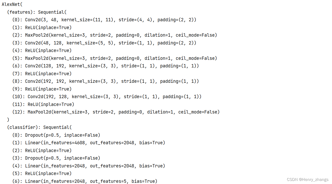
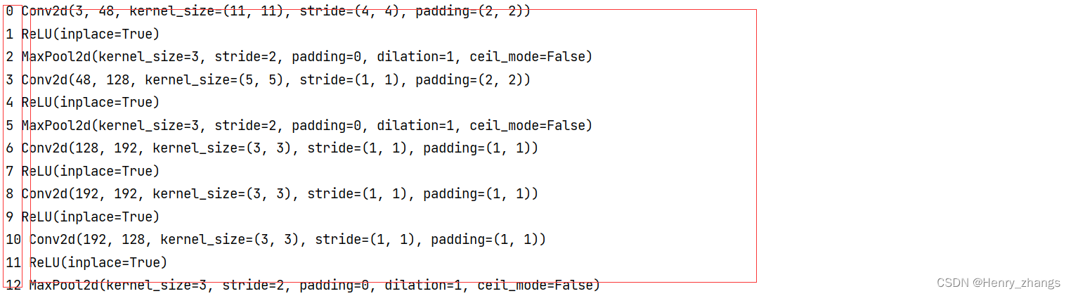
AlexNet网络的结构如图:
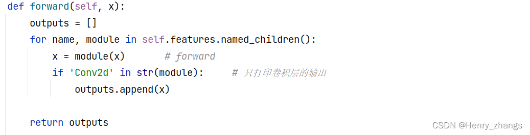
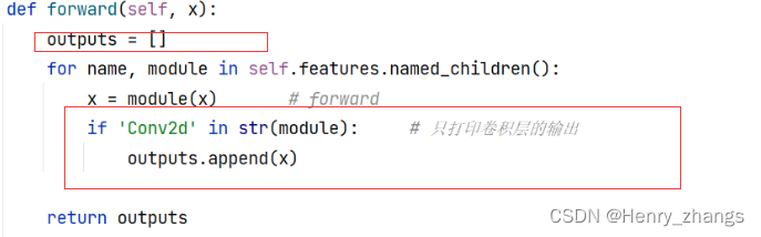
2.2 forward
这里AlexNet 网络的forward过程和之前定义的有所区别
如下:
这里的named_children() 会返回两个值,name是模块的名称,module是模块本身
调试信息如下:
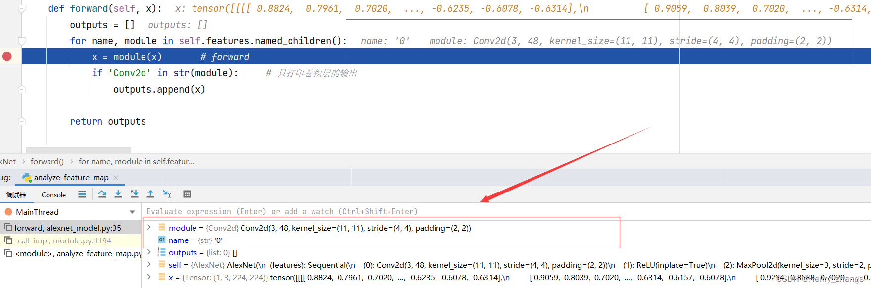
也就是说:name是第一个名称,module是第二个模块本身
所以这里的forward在features里面传递
注意这里没有classifier,这里是self.fetures里面的name_children
2.3 隐藏层特征图可视化
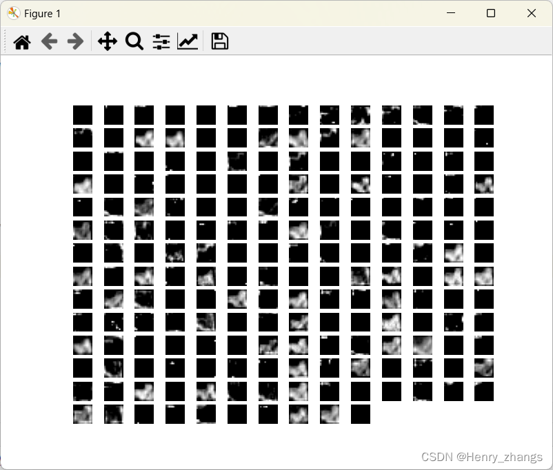
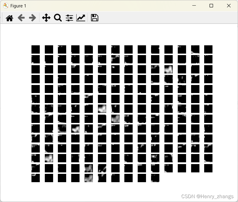
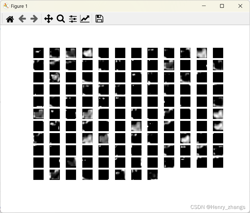
如图,这里将卷积层的输出保存在outputs里面,然后再return
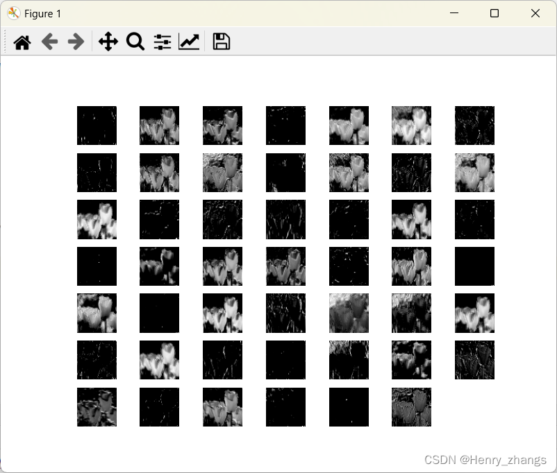
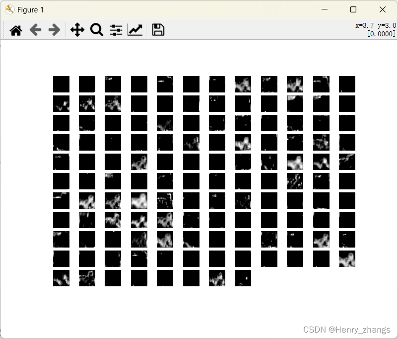
因为AlexNet 有五个卷积层,所以这里会显示五张特征图,如下:
2.4 测试代码
代码如下:
import os
os.environ['KMP_DUPLICATE_LIB_OK'] = 'True'
import torch
from alexnet_model import AlexNet
import matplotlib.pyplot as plt
import numpy as np
from PIL import Image
from torchvision import transforms
# 预处理
transformer = transforms.Compose([transforms.Resize((224, 224)), transforms.ToTensor(), transforms.Normalize((0.5, 0.5, 0.5), (0.5, 0.5, 0.5))])
# 实例化模型
model = AlexNet(num_classes=5)
model_weight_path = "./AlexNet.pth"
model.load_state_dict(torch.load(model_weight_path))
# load image
img = Image.open("./tulips.png")
img = transformer(img)
img = torch.unsqueeze(img, dim=0)
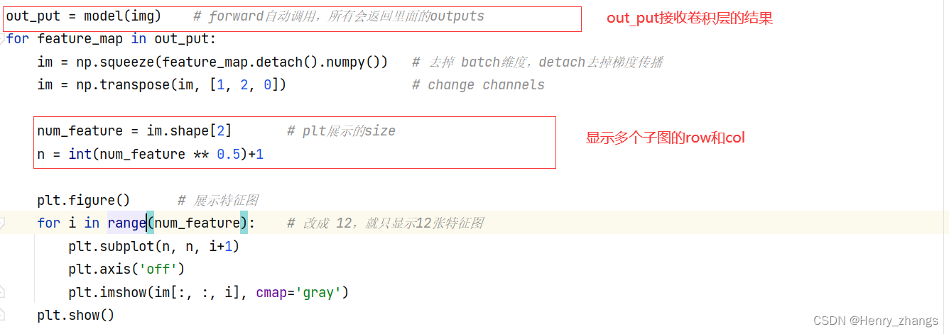
out_put = model(img) # forward自动调用,所有会返回里面的outputs
for feature_map in out_put:
im = np.squeeze(feature_map.detach().numpy()) # 去掉 batch维度,detach去掉梯度传播
im = np.transpose(im, [1, 2, 0]) # change channels
num_feature = im.shape[2] # plt展示的size
n = int(num_feature ** 0.5)+1
plt.figure() # 展示特征图
for i in range(num_feature): # 改成 12,就只显示12张特征图
plt.subplot(n, n, i+1)
plt.axis('off')
plt.imshow(im[:, :, i], cmap='gray')
plt.show()
其中:
model会自动调用里面的forward,因此直接接收返回值就行了
其次,这里将batch维度删去了,然后将channel返回到最后一个位置,所以打印的时候,需要将图像的每一个channel输出 im[: ,: ,i]
3. 训练参数的可视化
当模型训练好的时候,参数是可以显示的。这里可以将AlexNet 实例化,也可以不需要建立模型,直接从参数文件 .pth里面载入也可以。这里演示两种方法
3.1 从网络里面可视化参数
网络的结构如下
3.1.1 测试代码
代码:
import os
os.environ['KMP_DUPLICATE_LIB_OK'] = 'True'
import torch
from alexnet_model import AlexNet
import matplotlib.pyplot as plt
import numpy as np
# 实例化模型
model = AlexNet(num_classes=5)
model_weight_path = "./AlexNet.pth"
model.load_state_dict(torch.load(model_weight_path))
weights_keys = model.state_dict().keys() # 获取训练参数字典里面keys
for key in weights_keys:
# remove num_batches_tracked para(in bn)
if "num_batches_tracked" in key: # bn层也有参数
continue
# [卷积核个数,卷积核的深度, 卷积核 h,卷积核 w]
weight_value = model.state_dict()[key].numpy() # 返回 key 里面具体的值
# mean, std, min, max
weight_mean = weight_value.mean()
weight_std = weight_value.std()
weight_min = weight_value.min()
weight_max = weight_value.max()
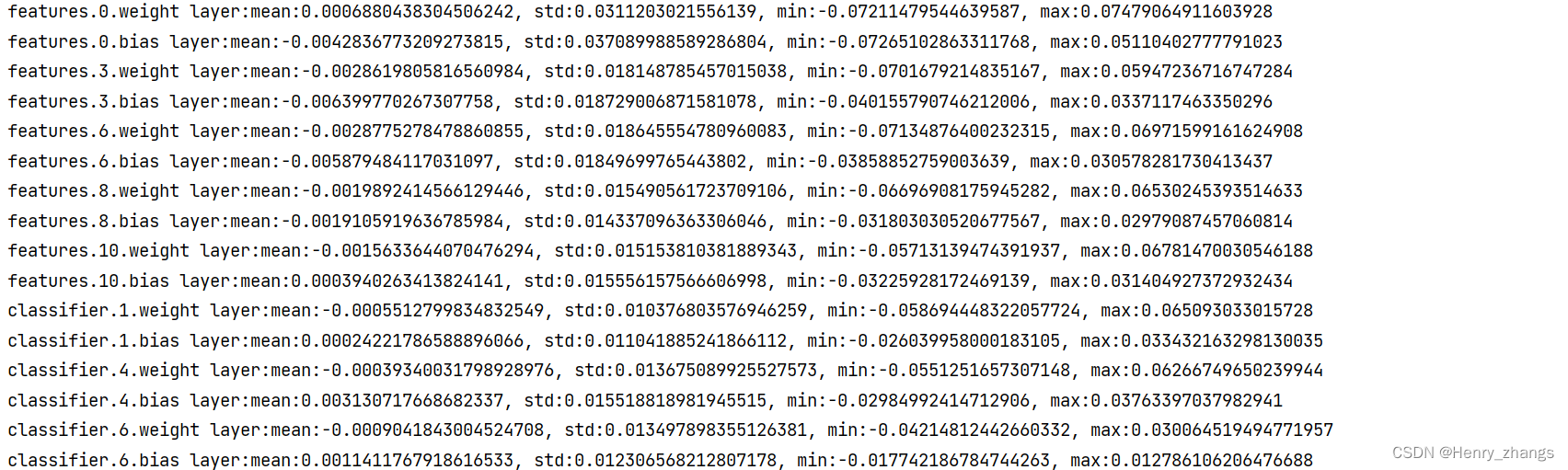
print("{} layer:mean:{}, std:{}, min:{}, max:{}".format(key,weight_mean,weight_std,weight_min,weight_max))
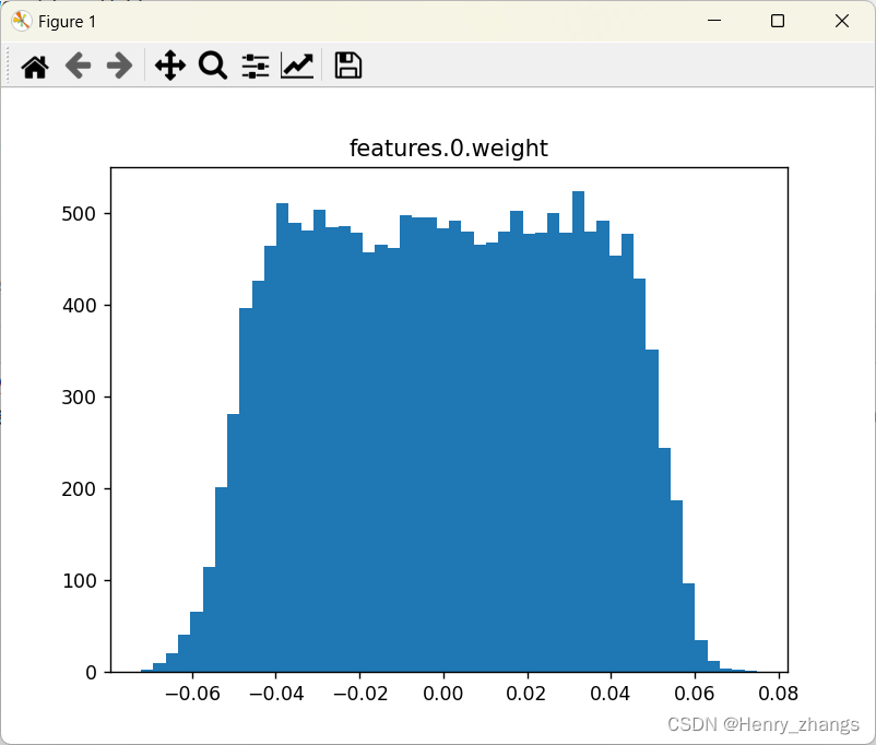
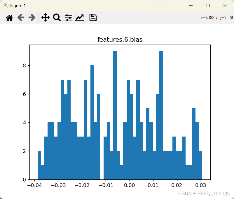
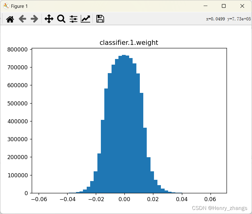
# 绘制参数的直方图
plt.close()
weight_vec = np.reshape(weight_value, [-1])
plt.hist(weight_vec, bins=50) # 将 min-max分成50份
plt.title(key)
plt.show()
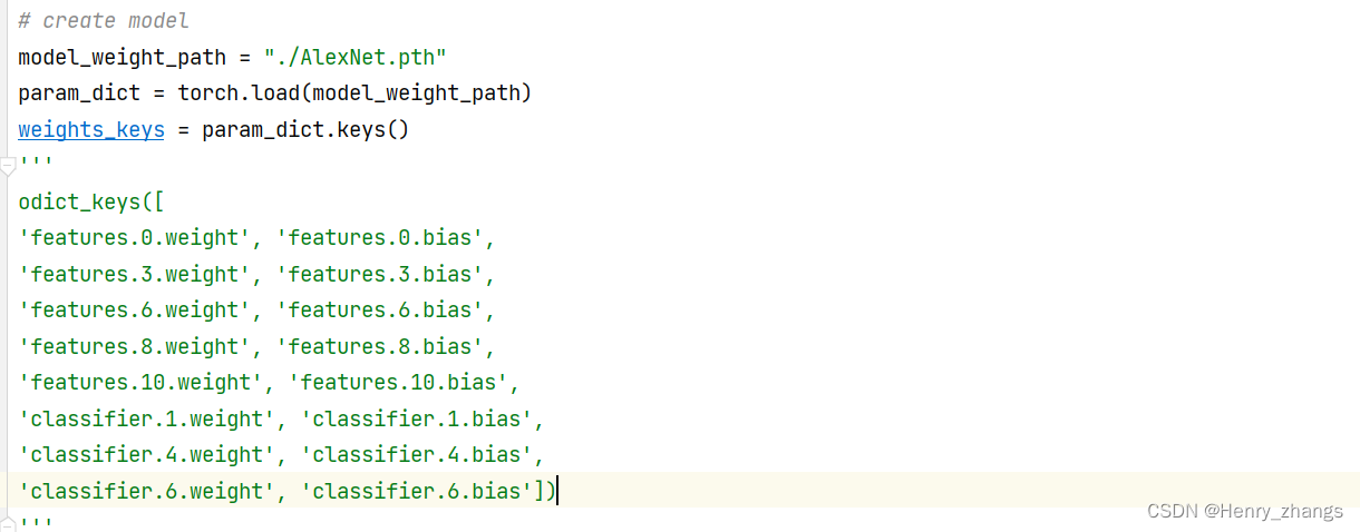
3.1.2 参数的字典信息
网络参数是一个字典存在的,这里打印里面的key值,
odcit(ordered dictionary) 是一个有序字典
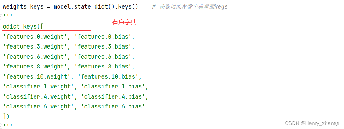
这里序号0,3,6....是因为网络只有这里层才有权重
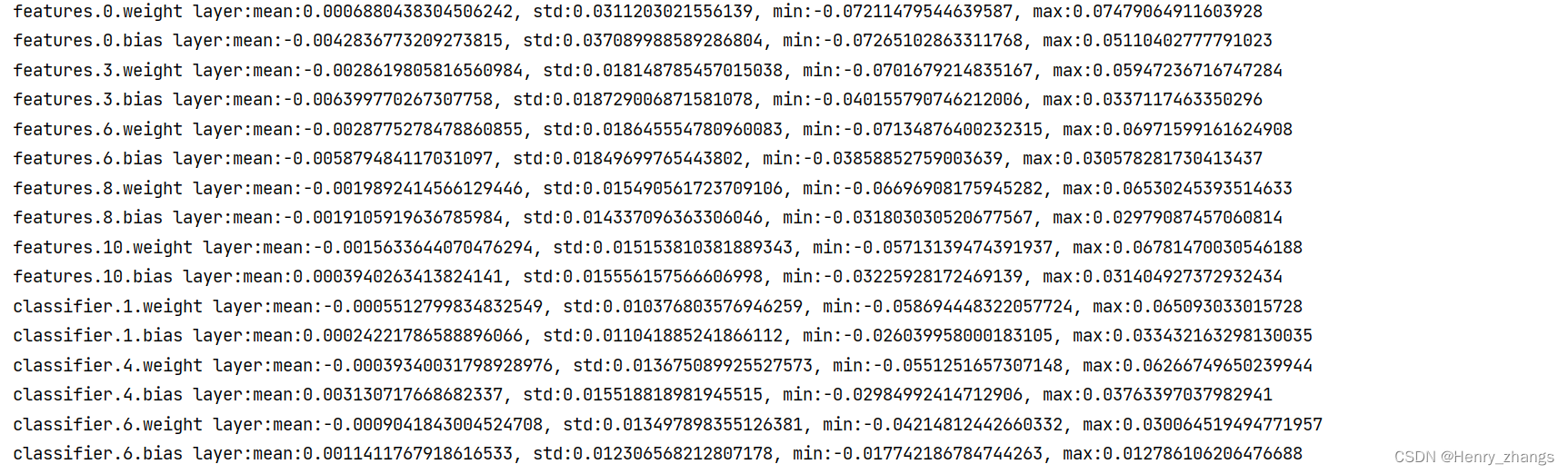
3.1.3 参数可视化
这里显示的有点多,所以只展示部分的

输出控制台的信息:
3.2 从保存的权重参数文件(.pth)里面可视化参数
代码:
import os
os.environ['KMP_DUPLICATE_LIB_OK'] = 'True'

import torch
import matplotlib.pyplot as plt
import numpy as np


# create model
model_weight_path = "./AlexNet.pth"
param_dict = torch.load(model_weight_path)
weights_keys = param_dict.keys()

for key in weights_keys:
    # remove num_batches_tracked para(in bn)
    if "num_batches_tracked" in key:
        continue

    # [卷积核个数,卷积核的深度, 卷积核 h,卷积核 w]
    weight_value = param_dict[key].numpy()

    # mean, std, min, max
    weight_mean = weight_value.mean()
    weight_std = weight_value.std()
    weight_min = weight_value.min()
    weight_max = weight_value.max()
    print("{} layer:mean:{}, std:{}, min:{}, max:{}".format(key,weight_mean,weight_std,weight_min,weight_max))

    # 绘制参数的直方图
    plt.close()
    weight_vec = np.reshape(weight_value, [-1])
    plt.hist(weight_vec, bins=50)   # 将 min-max分成50份
    plt.title(key)
    plt.show()
其中载入参数的字典文件如下:
打印的信息: