工具系列：TimeGPT_(8)使用不规则时间戳进行时间序列预测

介绍

在处理时间序列数据时，时间戳的频率是一个关键因素，可以对预测结果产生重大影响。像每日、每周或每月这样的常规频率很容易处理。然而，像工作日这样的不规则频率（不包括周末）对于时间序列预测方法来说可能是具有挑战性的。

我们的预测方法可以处理这种不规则的时间序列数据，只要您指定了序列的频率。例如，在工作日的情况下，频率应该传递为’B’。如果没有这个参数，方法可能无法自动检测频率，特别是当时间戳是不规则的时候。

# Import the colab_badge module from the nixtlats.utils package
from nixtlats.utils import colab_badge

colab_badge('docs/tutorials/8_irregular_timestamps')

from fastcore.test import test_eq, test_fail, test_warns
from dotenv import load_dotenv

# 导入load_dotenv函数，用于加载.env文件中的环境变量
load_dotenv()

True

# 导入pandas库，用于数据处理
import pandas as pd

# 导入TimeGPT模块
from nixtlats import TimeGPT

/home/ubuntu/miniconda/envs/nixtlats/lib/python3.11/site-packages/statsforecast/core.py:25: TqdmWarning: IProgress not found. Please update jupyter and ipywidgets. See https://ipywidgets.readthedocs.io/en/stable/user_install.html
  from tqdm.autonotebook import tqdm

# 创建一个TimeGPT对象，并传入一个参数token，用于验证身份
# 如果没有提供token参数，则默认使用环境变量中的TIMEGPT_TOKEN

timegpt = TimeGPT(
    token = 'my_token_provided_by_nixtla'
)

# 导入TimeGPT模型

timegpt = TimeGPT()  # 创建TimeGPT对象的实例

不规则时间戳的单变量时间预测

第一步是获取您的时间序列数据。数据必须包括时间戳和相关的值。例如，您可能正在处理股票价格，您的数据可能如下所示。在这个例子中，我们使用OpenBB。

# 从指定URL读取数据集
df_fed_test = pd.read_csv('https://raw.githubusercontent.com/Nixtla/transfer-learning-time-series/main/datasets/openbb/fed.csv')

# 使用pd.testing.assert_frame_equal函数对两个预测结果进行比较
# 第一个预测结果使用默认的频率（每日）
# 第二个预测结果使用频率为每周
# 比较的指标为预测结果的FF列，并设置置信水平为90%
pd.testing.assert_frame_equal(
    timegpt.forecast(df_fed_test, h=12, target_col='FF', level=[90]),
    timegpt.forecast(df_fed_test, h=12, target_col='FF', freq='W', level=[90])
)

INFO:nixtlats.timegpt:Validating inputs...
INFO:nixtlats.timegpt:Preprocessing dataframes...
INFO:nixtlats.timegpt:Inferred freq: W-WED
WARNING:nixtlats.timegpt:The specified horizon "h" exceeds the model horizon. This may lead to less accurate forecasts. Please consider using a smaller horizon.
INFO:nixtlats.timegpt:Restricting input...
INFO:nixtlats.timegpt:Calling Forecast Endpoint...
INFO:nixtlats.timegpt:Validating inputs...
INFO:nixtlats.timegpt:Preprocessing dataframes...
INFO:nixtlats.timegpt:Inferred freq: W-WED
WARNING:nixtlats.timegpt:The specified horizon "h" exceeds the model horizon. This may lead to less accurate forecasts. Please consider using a smaller horizon.
INFO:nixtlats.timegpt:Restricting input...
INFO:nixtlats.timegpt:Calling Forecast Endpoint...

# 从指定的URL读取CSV文件，并将其存储在名为pltr_df的DataFrame中
pltr_df = pd.read_csv('https://raw.githubusercontent.com/Nixtla/transfer-learning-time-series/main/datasets/openbb/pltr.csv')

# 将'date'列转换为日期时间格式，并将结果存储在'date'列中
pltr_df['date'] = pd.to_datetime(pltr_df['date'])

# 显示数据集的前几行
pltr_df.head()

	date	Open	High	Low	Close	Adj Close	Volume	Dividends	Stock Splits
0	2020-09-30	10.00	11.41	9.11	9.50	9.50	338584400	0.0	0.0
1	2020-10-01	9.69	10.10	9.23	9.46	9.46	124297600	0.0	0.0
2	2020-10-02	9.06	9.28	8.94	9.20	9.20	55018300	0.0	0.0
3	2020-10-05	9.43	9.49	8.92	9.03	9.03	36316900	0.0	0.0
4	2020-10-06	9.04	10.18	8.90	9.90	9.90	90864000	0.0	0.0

让我们看看这个数据集有不规则的时间戳。来自pandas的DatetimeIndex的dayofweek属性返回星期几，星期一=0，星期日=6。因此，检查dayofweek>4实际上是检查日期是否落在周六（5）或周日（6），这通常是非工作日（周末）。

# 统计pltr_df中日期的星期几大于4的数量
(pltr_df['date'].dt.dayofweek > 4).sum()

0

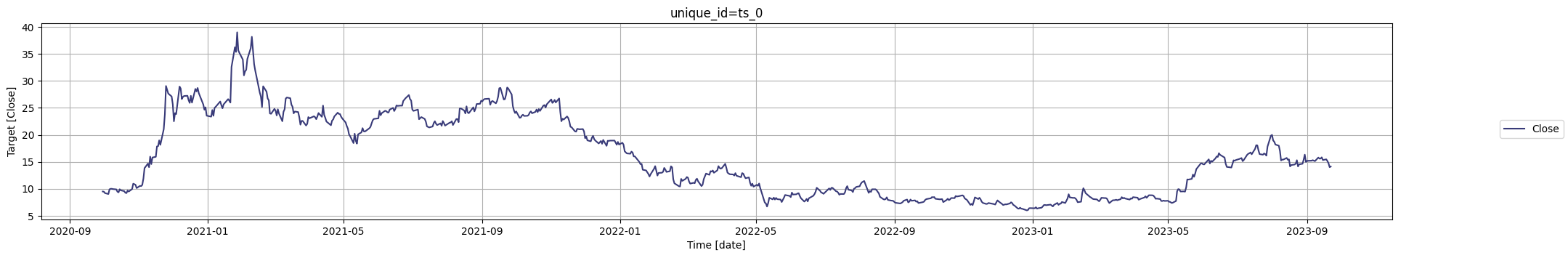
我们可以看到时间戳是不规则的。让我们检查“Close”系列。

# 使用timegpt模块中的plot函数，绘制pltr_df数据集中的日期(date)与收盘价(Close)之间的关系图
timegpt.plot(pltr_df, time_col='date', target_col='Close')

要预测这些数据，您可以使用我们的forecast方法。重要的是，记得使用freq参数指定数据的频率。在这种情况下，它应该是’B’，表示工作日。我们还需要定义time_col来选择系列的索引（默认为ds），以及target_col来预测我们的目标变量，这种情况下我们将预测Close。

# 预测函数test_fail()用于测试timegpt.forecast()函数的功能
# timegpt.forecast()函数用于根据给定的时间序列数据进行预测
# 该函数的参数包括：
# - df：时间序列数据的DataFrame
# - h：预测的时间步数
# - time_col：时间列的名称
# - target_col：目标列的名称

# 在这个测试中，我们使用pltr_df作为输入数据进行预测
# 预测的时间步数为14
# 时间列的名称为'date'
# 目标列的名称为'Close'

# 预测结果中应该包含'frequency'，但是由于某种原因，预测失败了
test_fail(
    lambda: timegpt.forecast(
        df=pltr_df, h=14,
        time_col='date', target_col='Close',
    ),
    contains='frequency'
)

INFO:nixtlats.timegpt:Validating inputs...
INFO:nixtlats.timegpt:Preprocessing dataframes...

# 导入所需的模块和函数


# 调用forecast函数，传入时间序列数据的DataFrame、预测步长、频率、时间列的列名和目标列的列名
fcst_pltr_df = timegpt.forecast(
    df=pltr_df, h=14, freq='B',
    time_col='date', target_col='Close',
)

INFO:nixtlats.timegpt:Validating inputs...
INFO:nixtlats.timegpt:Preprocessing dataframes...
WARNING:nixtlats.timegpt:The specified horizon "h" exceeds the model horizon. This may lead to less accurate forecasts. Please consider using a smaller horizon.
INFO:nixtlats.timegpt:Calling Forecast Endpoint...

# 查看数据集的前几行
fcst_pltr_df.head()

	date	TimeGPT
0	2023-09-25	14.688427
1	2023-09-26	14.742798
2	2023-09-27	14.781240
3	2023-09-28	14.824156
4	2023-09-29	14.795214

记住，对于工作日，频率是’B’。对于其他频率，您可以参考pandas偏移别名文档：https://pandas.pydata.org/pandas-docs/stable/user_guide/timeseries.html#timeseries-offset-aliases。

通过指定频率，您可以帮助预测方法更好地理解数据中的模式，从而得到更准确可靠的预测结果。

让我们绘制由TimeGPT生成的预测结果。

# 使用timegpt.plot函数绘制图表
# 参数pltr_df是包含股票价格数据的DataFrame
# 参数fcst_pltr_df是包含预测股票价格数据的DataFrame
# 参数time_col指定时间列的名称，这里是'date'
# 参数target_col指定目标列的名称，这里是'Close'
# 参数max_insample_length指定用于训练模型的最大样本数量，这里是90
timegpt.plot(
    pltr_df, 
    fcst_pltr_df, 
    time_col='date',
    target_col='Close',
    max_insample_length=90, 
)

您还可以使用level参数将不确定性量化添加到您的预测中。

# 导入所需的模块和函数

# 使用timegpt.forecast函数进行时间序列预测
# 参数df为输入的数据框，pltr_df为待预测的数据框
# 参数h为预测的时间步长，这里设置为42
# 参数freq为数据的频率，这里设置为工作日（B）
# 参数time_col为时间列的名称，这里设置为'date'
# 参数target_col为目标列的名称，这里设置为'Close'
# 参数add_history为是否将历史数据添加到预测结果中，这里设置为True
# 参数level为置信水平，这里设置为[40.66, 90]
fcst_pltr_levels_df = timegpt.forecast(
    df=pltr_df, h=42, freq='B',
    time_col='date', target_col='Close',
    add_history=True,
    level=[40.66, 90],
)

INFO:nixtlats.timegpt:Validating inputs...
INFO:nixtlats.timegpt:Preprocessing dataframes...
WARNING:nixtlats.timegpt:The specified horizon "h" exceeds the model horizon. This may lead to less accurate forecasts. Please consider using a smaller horizon.
INFO:nixtlats.timegpt:Calling Forecast Endpoint...
INFO:nixtlats.timegpt:Calling Historical Forecast Endpoint...

# 绘制时间序列图
# 参数：
# pltr_df: 包含时间序列数据的DataFrame
# fcst_pltr_levels_df: 包含预测水平数据的DataFrame
# time_col: 时间列的列名
# target_col: 目标列的列名
# level: 预测水平的取值范围
timegpt.plot(
    pltr_df, 
    fcst_pltr_levels_df, 
    time_col='date',
    target_col='Close',
    level=[40.66, 90],
)

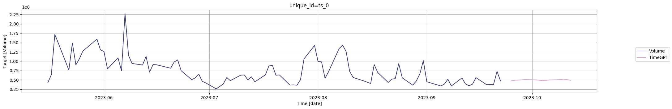
如果你想预测另一个变量，只需更改“target_col”参数。现在让我们预测“Volume”：

# 导入所需模块和函数

# 使用timegpt.forecast函数进行时间序列预测
# 参数df为输入的时间序列数据，pltr_df为输入的数据框
# 参数h为预测的步长，这里设置为14
# 参数freq为时间序列的频率，这里设置为'B'，表示工作日
# 参数time_col为时间列的名称，这里设置为'date'
# 参数target_col为目标列的名称，这里设置为'Volume'
fcst_pltr_df = timegpt.forecast(
    df=pltr_df, h=14, freq='B',
    time_col='date', target_col='Volume',
)

# 使用timegpt.plot函数绘制时间序列和预测结果的图形
# 参数pltr_df为输入的时间序列数据，这里是原始数据
# 参数fcst_pltr_df为预测结果数据，这里是预测的结果
# 参数time_col为时间列的名称，这里设置为'date'
# 参数max_insample_length为显示的最大样本长度，这里设置为90
# 参数target_col为目标列的名称，这里设置为'Volume'
timegpt.plot(
    pltr_df, 
    fcst_pltr_df, 
    time_col='date',
    max_insample_length=90,
    target_col='Volume',
)

INFO:nixtlats.timegpt:Validating inputs...
INFO:nixtlats.timegpt:Preprocessing dataframes...
WARNING:nixtlats.timegpt:The specified horizon "h" exceeds the model horizon. This may lead to less accurate forecasts. Please consider using a smaller horizon.
INFO:nixtlats.timegpt:Calling Forecast Endpoint...

但是如果我们想同时预测所有时间序列呢？我们可以通过重新塑造我们的数据框来实现。目前，数据框是宽格式（每个序列是一列），但我们需要将它们转换为长格式（一个接一个地堆叠）。我们可以使用以下方式实现：

# 将pltr_df进行重塑，使得每一行代表一个观测值
# id_vars参数指定date列为标识变量，即不需要重塑的列
# var_name参数指定新生成的列名为series_id
pltr_long_df = pd.melt(
    pltr_df, 
    id_vars=['date'],
    var_name='series_id'
)

# 显示数据集的前几行
pltr_long_df.head()

	date	series_id	value
0	2020-09-30	Open	10.00
1	2020-10-01	Open	9.69
2	2020-10-02	Open	9.06
3	2020-10-05	Open	9.43
4	2020-10-06	Open	9.04

然后我们只需简单地调用forecast方法，并指定id_col参数。

# 导入所需的模块和函数已在代码中，无需额外的import语句

# 调用timegpt模块中的forecast函数，对pltr_long_df数据进行预测
# 参数df表示要进行预测的数据框，pltr_long_df为待预测的数据框
# 参数h表示预测的时间步数，这里设置为14，即预测未来14个时间步的值
# 参数freq表示数据的频率，这里设置为'B'，表示工作日频率
# 参数id_col表示数据框中表示序列ID的列名，这里设置为'series_id'
# 参数time_col表示数据框中表示时间的列名，这里设置为'date'
# 参数target_col表示数据框中表示目标变量的列名，这里设置为'value'
fcst_pltr_long_df = timegpt.forecast(
    df=pltr_long_df, h=14, freq='B',
    id_col='series_id', time_col='date', target_col='value',
)

INFO:nixtlats.timegpt:Validating inputs...
INFO:nixtlats.timegpt:Preprocessing dataframes...
WARNING:nixtlats.timegpt:The specified horizon "h" exceeds the model horizon. This may lead to less accurate forecasts. Please consider using a smaller horizon.
INFO:nixtlats.timegpt:Calling Forecast Endpoint...

# 显示 DataFrame 的前五行数据
fcst_pltr_long_df.head()

	series_id	date	TimeGPT
0	Adj Close	2023-09-25	14.688427
1	Adj Close	2023-09-26	14.742798
2	Adj Close	2023-09-27	14.781240
3	Adj Close	2023-09-28	14.824156
4	Adj Close	2023-09-29	14.795214

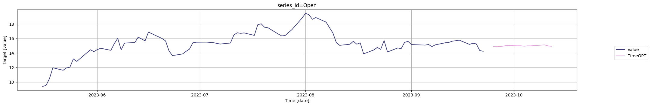
然后我们可以预测“开盘价”系列：

# 使用timegpt.plot函数绘制图表
# 参数pltr_long_df是包含原始数据的DataFrame
# 参数fcst_pltr_long_df是包含预测数据的DataFrame
# 参数id_col指定数据中用于标识系列的列名
# 参数time_col指定数据中用于表示时间的列名
# 参数target_col指定数据中用于表示目标值的列名
# 参数unique_ids是一个列表，包含需要绘制图表的唯一系列的标识符
# 参数max_insample_length指定用于训练模型的最大样本长度
timegpt.plot(
    pltr_long_df, 
    fcst_pltr_long_df, 
    id_col='series_id',
    time_col='date',
    target_col='value',
    unique_ids=['Open'],
    max_insample_length=90,
)

不规则时间戳的外生变量时间预测

在时间序列预测中，我们预测的变量通常不仅受到它们过去的值的影响，还受到其他因素或变量的影响。这些外部变量被称为外生变量，它们可以提供重要的额外背景信息，可以显著提高我们的预测准确性。其中一个因素，也是本教程的重点，是公司的营收。营收数据可以提供公司财务健康和增长潜力的关键指标，这两者都可以对其股票价格产生重大影响。我们可以从openbb获取这些数据。

# 从指定的 URL 中读取 CSV 文件，并将其存储在名为 revenue_pltr 的数据框中
revenue_pltr = pd.read_csv('https://raw.githubusercontent.com/Nixtla/transfer-learning-time-series/main/datasets/openbb/revenue-pltr.csv')

# 获取revenue_pltr中'totalRevenue'列的第一个值
value = revenue_pltr['totalRevenue'].iloc[0]

# 判断value是否为float类型且包含'M'
if not isinstance(value, float) and 'M' in value:
    
    # 定义一个函数convert_to_float，用于将字符串转换为浮点数
    def convert_to_float(val):
        # 如果val中包含'M'，则将'M'替换为空字符串，并将结果乘以1e6（表示百万）
        if 'M' in val:
            return float(val.replace(' M', '')) * 1e6
        # 如果val中包含'K'，则将'K'替换为空字符串，并将结果乘以1e3（表示千）
        elif 'K' in val:
            return float(val.replace(' K', '')) * 1e3
        # 如果val中既不包含'M'也不包含'K'，则直接将val转换为浮点数
        else:
            return float(val)
    
    # 将'revenue_pltr'中'totalRevenue'列的每个值都应用convert_to_float函数进行转换
    revenue_pltr['totalRevenue'] = revenue_pltr['totalRevenue'].apply(convert_to_float)

# 显示数据的最后几行
revenue_pltr.tail()

	fiscalDateEnding	totalRevenue
5	2022-06-30	473010000.0
6	2022-09-30	477880000.0
7	2022-12-31	508624000.0
8	2023-03-31	525186000.0
9	2023-06-30	533317000.0

我们在数据集中观察到的第一件事是，我们只能获得到2023年第一季度结束的信息。我们的数据以季度频率表示，我们的目标是利用这些信息来预测超过这个日期的未来14天的每日股票价格。

然而，为了准确计算包括收入作为外生变量的这种预测，我们需要了解未来收入的值。这是至关重要的，因为这些未来收入值可以显著影响股票价格。

由于我们的目标是预测未来14天的每日股票价格，我们只需要预测即将到来的一个季度的收入。这种方法使我们能够创建一个连贯的预测流程，其中一个预测的输出（收入）被用作另一个预测（股票价格）的输入，从而利用所有可用的信息以获得最准确的预测。

# 定义一个变量fcst_pltr_revenue，用于存储预测结果
# 调用timegpt库中的forecast函数，对revenue_pltr数据进行预测
# 预测的时间跨度为1，时间列为fiscalDateEnding，目标列为totalRevenue
fcst_pltr_revenue = timegpt.forecast(revenue_pltr, h=1, time_col='fiscalDateEnding', target_col='totalRevenue')

INFO:nixtlats.timegpt:Validating inputs...
INFO:nixtlats.timegpt:Preprocessing dataframes...
INFO:nixtlats.timegpt:Inferred freq: Q-DEC
INFO:nixtlats.timegpt:Calling Forecast Endpoint...

# 查看数据集的前几行
fcst_pltr_revenue.head()

	fiscalDateEnding	TimeGPT
0	2023-09-30	540005888

继续上次的内容，我们预测流程中的下一个关键步骤是调整数据的频率，以匹配股票价格的频率，股票价格的频率是以工作日为基准的。为了实现这一点，我们需要对历史和未来预测的收入数据进行重新采样。

我们可以使用以下代码来实现这一点

# 将'revenue_pltr'数据框中的'fiscalDateEnding'列转换为日期格式
revenue_pltr['fiscalDateEnding'] = pd.to_datetime(revenue_pltr['fiscalDateEnding'])
revenue_pltr = revenue_pltr.set_index('fiscalDateEnding').resample('B').ffill().reset_index()

重要提示：需要强调的是，在这个过程中，我们将相同的收入值分配给给定季度内的所有天数。这种简化是必要的，因为季度收入数据和每日股票价格数据之间的粒度差异很大。然而，在实际应用中，对这个假设要谨慎对待是至关重要的。季度收入数据对每日股票价格的影响在季度内可以根据一系列因素（包括市场预期的变化、其他财经新闻和事件）而有很大的差异。在本教程中，我们使用这个假设来说明如何将外部变量纳入我们的预测模型，但在实际情况下，根据可用数据和具体用例，可能需要采用更细致的方法。

然后我们可以创建完整的历史数据集。

# 合并数据框
# 将revenue_pltr数据框的'fiscalDateEnding'列重命名为'date'列，并与pltr_df数据框进行合并
pltr_revenue_df = pltr_df.merge(revenue_pltr.rename(columns={
    
    'fiscalDateEnding': 'date'}))

# 显示DataFrame的前几行数据
pltr_revenue_df.head()

	date	Open	High	Low	Close	Adj Close	Volume	Dividends	Stock Splits	totalRevenue
0	2021-03-31	22.500000	23.850000	22.379999	23.290001	23.290001	61458500	0.0	0.0	341234000.0
1	2021-04-01	23.950001	23.950001	22.730000	23.070000	23.070000	51788800	0.0	0.0	341234000.0
2	2021-04-05	23.780001	24.450001	23.340000	23.440001	23.440001	65374300	0.0	0.0	341234000.0
3	2021-04-06	23.549999	23.610001	22.830000	23.270000	23.270000	41933500	0.0	0.0	341234000.0
4	2021-04-07	23.000000	23.549999	22.809999	22.900000	22.900000	32766200	0.0	0.0	341234000.0

计算未来收入的数据框架：

# 设置变量horizon为14，表示水平线的位置为14
horizon = 14

# 导入numpy库，用于进行科学计算和数组操作
import numpy as np

# 创建一个DataFrame对象future_df
# 该DataFrame包含两列：'date'和'totalRevenue'
# 'date'列使用pd.date_range函数生成，从pltr_revenue_df的最后一个日期开始，生成horizon + 1个日期，频率为工作日（'B'）
# 从生成的日期中取出后horizon个日期，作为'future_df'的'date'列
# 'totalRevenue'列使用np.repeat函数生成，将fcst_pltr_revenue的第一个元素的'TimeGPT'值重复horizon次
future_df = pd.DataFrame({
    
    
    'date': pd.date_range(pltr_revenue_df['date'].iloc[-1], periods=horizon + 1, freq='B')[-horizon:],
    'totalRevenue': np.repeat(fcst_pltr_revenue.iloc[0]['TimeGPT'], horizon)
})

# 查看数据集的前几行
future_df.head()

	date	totalRevenue
0	2023-07-03	540005888
1	2023-07-04	540005888
2	2023-07-05	540005888
3	2023-07-06	540005888
4	2023-07-07	540005888

然后，我们可以使用X_df参数在forecast方法中传递未来的收入。由于收入在历史数据框中，该信息将被用于模型中。

# 使用timegpt模块中的forecast函数，对pltr_revenue_df数据进行预测
# 预测的时间范围为horizon
# 频率为'B'，即每个工作日
# 时间列为'date'
# 目标列为'Close'
# 附加的特征数据为future_df
fcst_pltr_df = timegpt.forecast(
    pltr_revenue_df, h=horizon, 
    freq='B',
    time_col='date', 
    target_col='Close',
    X_df=future_df,
)

INFO:nixtlats.timegpt:Validating inputs...
INFO:nixtlats.timegpt:Preprocessing dataframes...
WARNING:nixtlats.timegpt:The specified horizon "h" exceeds the model horizon. This may lead to less accurate forecasts. Please consider using a smaller horizon.
INFO:nixtlats.timegpt:Calling Forecast Endpoint...

# 绘制时间序列预测图
# 参数说明：
# pltr_revenue_df: 公司收入数据的DataFrame
# fcst_pltr_df: 预测的公司收入数据的DataFrame
# id_col: 数据中表示系列ID的列名
# time_col: 数据中表示时间的列名
# target_col: 数据中表示目标变量的列名
# max_insample_length: 用于训练模型的最大样本长度
timegpt.plot(
    pltr_revenue_df, 
    fcst_pltr_df, 
    id_col='series_id',
    time_col='date',
    target_col='Close',
    max_insample_length=90,
)

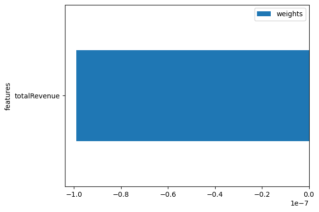
我们还可以看到收入的重要性。

timegpt.weights_x.plot.barh(x='features', y='weights')

<Axes: ylabel='features'>