吴恩达机器学习作业（4）：正则化逻辑回归

1）数据可视化

2）创建多项式特征

3）正则化成本函数

4）正则化梯度下降

4）准确度

5）Scikit-learn实现

正则化是成本函数中的一个术语，它使算法更倾向于“更简单”的模型（在这种情况下，模型将有更小的系数）。这个理论有助于减少过拟合，提高模型的泛化能力。这样，我们开始吧。

设想你是工厂的生产主管，你有一些芯片在两次测试中的测试结果。对于这两次测试，你想决定是否芯片要被接受或抛弃。为了帮助你做出艰难的决定，你拥有过去芯片的测试数据集，从其中你可以构建一个逻辑回归模型。

和第一部分很像，从数据可视化开始吧！

1）数据可视化

我们这里使用之前导入过的库：

path =  'ex2data2.txt'
data2 = pd.read_csv(path, header=None, names=['Test 1', 'Test 2', 'Accepted'])
data2.head()

positive = data2[data2['Accepted'].isin([1])]
negative = data2[data2['Accepted'].isin([0])]

fig, ax = plt.subplots(figsize=(12,8))
ax.scatter(positive['Test 1'], positive['Test 2'], s=50, c='b', marker='o', label='Accepted')
ax.scatter(negative['Test 1'], negative['Test 2'], s=50, c='r', marker='x', label='Rejected')
ax.legend()
ax.set_xlabel('Test 1 Score')
ax.set_ylabel('Test 2 Score')
plt.show()

这个数据看起来可比前一次的复杂得多。特别地，你会注意到其中没有线性决策界限，来良好的分开两类数据。一个方法是用像逻辑回归这样的线性技术来构造从原始特征的多项式中得到的特征。让我们通过创建一组多项式特征入手吧。

2）创建多项式特征

degree = 5
x1 = data2['Test 1']
x2 = data2['Test 2']

data2.insert(3, 'Ones', 1)

for i in range(1, degree):
    for j in range(0, i):
        data2['F' + str(i) + str(j)] = np.power(x1, i-j) * np.power(x2, j)

data2.drop('Test 1', axis=1, inplace=True)
data2.drop('Test 2', axis=1, inplace=True)

data2.head()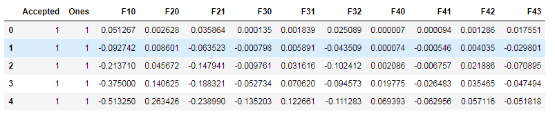

3）正则化成本函数

$J\left( \theta \right)=\frac{1}{m}\sum\limits_{i=1}^{m}{[-{{y}^{(i)}}\log \left( {{h}_{\theta }}\left( {{x}^{(i)}} \right) \right)-\left( 1-{{y}^{(i)}} \right)\log \left( 1-{{h}_{\theta }}\left( {{x}^{(i)}} \right) \right)]}+\frac{\lambda }{2m}\sum\limits_{j=1}^{n}{\theta _{j}^{2}}$

def costReg(theta, X, y, learningRate):
    theta = np.matrix(theta)
    X = np.matrix(X)
    y = np.matrix(y)
    first = np.multiply(-y, np.log(sigmoid(X * theta.T)))
    second = np.multiply((1 - y), np.log(1 - sigmoid(X * theta.T)))
    reg = (learningRate / (2 * len(X))) * np.sum(np.power(theta[:,1:theta.shape[1]], 2))
    return np.sum(first - second) / len(X) + reg

4）正则化梯度下降

现在我们来看看正则化的代价函数，只是第一项未正则化：

$\theta_0:=\theta_0-\alpha\frac{1}{m}\sum_{i=1}^{m}[h_\theta(x^{(i)})-y^{(i)}]x_0^{(i)}$

$\theta_j:=\theta_j-\alpha\frac{1}{m}\sum_{i=1}^{m}[h_\theta(x^{(i)})-y^{(i)}]x_j^{(i)}+\frac{\lambda}{m}\theta_j$

对上面的算法中 j=1,2,...,n 时的更新式子进行调整可得：

${{\theta }_{j}}:={{\theta }_{j}}(1-a\frac{\lambda }{m})-a\frac{1}{m}\sum\limits_{i=1}^{m}{({{h}_{\theta }}\left( {{x}^{(i)}} \right)-{{y}^{(i)}})x_{j}^{(i)}}$

def gradientReg(theta, X, y, learningRate):
    theta = np.matrix(theta)
    X = np.matrix(X)
    y = np.matrix(y)
    
    parameters = int(theta.ravel().shape[1])
    grad = np.zeros(parameters)
    
    error = sigmoid(X * theta.T) - y
    
    for i in range(parameters):
        term = np.multiply(error, X[:,i])
        
        if (i == 0):
            grad[i] = np.sum(term) / len(X)
        else:
            grad[i] = (np.sum(term) / len(X)) + ((learningRate / len(X)) * theta[:,i])
    
    return grad

4）准确度

剩下的操作就像之前一样：

# set X and y (remember from above that we moved the label to column 0)
cols = data2.shape[1]
X2 = data2.iloc[:,1:cols]
y2 = data2.iloc[:,0:1]

# convert to numpy arrays and initalize the parameter array theta
X2 = np.array(X2.values)
y2 = np.array(y2.values)
theta2 = np.zeros(11)

learningRate = 1

现在，我们来计算新的默认为0的正则化函数的值：

costReg(theta2, X2, y2, learningRate)

0.6931471805599454

gradientReg(theta2, X2, y2, learningRate)

array([0.00847458, 0.01878809, 0.05034464, 0.01150133, 0.01835599,
       0.00732393, 0.00819244, 0.03934862, 0.00223924, 0.01286005,
       0.00309594])

现在我们可以使用和第一部分相同的优化函数来计算优化后的结果。

result2 = opt.fmin_tnc(func=costReg, x0=theta2, fprime=gradientReg, args=(X2, y2, learningRate))
result2

(array([  1.22702519e-04,   7.19894617e-05,  -3.74156201e-04,
         -1.44256427e-04,   2.93165088e-05,  -5.64160786e-05,
         -1.02826485e-04,  -2.83150432e-04,   6.47297947e-07,
         -1.99697568e-04,  -1.68479583e-05]), 96, 1)

最后，我们可以使用第1部分中的预测函数来查看我们的方案在训练数据上的准确度。

theta_min = np.matrix(result2[0])
predictions = predict(theta_min, X2)
correct = [1 if ((a == 1 and b == 1) or (a == 0 and b == 0)) else 0 for (a, b) in zip(predictions, y2)]
accuracy = (sum(map(int, correct)) % len(correct))
print ('accuracy = {0}%'.format(accuracy))

5）Scikit-learn实现

from sklearn import linear_model#调用sklearn的线性回归包
model = linear_model.LogisticRegression(penalty='l2', C=1.0)
model.fit(X2, y2.ravel())

model.score(X2, y2)
0.6610169491525424

这个准确度和我们刚刚实现的差了好多，不过请记住这个结果是使用默认参数下计算的结果。我们可能需要做一些参数的调整来获得和我们之前结果相同的精确度。