洛伦兹方程

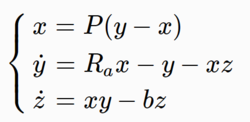
洛伦兹方程(Lorenz equation)描述空气流体 运动的一个简化微分方程组.1963年，美国气象学家洛伦兹(Lorenz,E. N.)将描述大气热对流的非线 性偏微分方程组通过傅里叶展开，大胆地截断而导 出描述垂直速度、上下温差的展开系数x(t),y(t),z(t)的三维自治动力系统

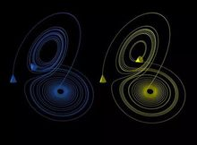
其中，P:为普朗特数，Ra为瑞利数.他发现当Ra 不断增加时，系统就由定常态(表示空气静止)分岔 出周期态(表示对流状态)，最后，当Ra>24. 74时， 又分岔出非周期的混沌态(表示湍流).如图是三维相空间的混沌态在二维平面上的投影轨线.从图上 看出，轨线起初在右边从外向内绕圈子，后来随机地 跳到左边从外向内绕圈子，后又再次随机地跳回右边绕圈子，……如此左右跳来跳去，每次绕的圈数，何时发生跳跃都是随机的、无规则的. 由于洛伦兹是世界上第一个从确定的方程中发现了非周期的混沌现象，所以将上述方程一般称为洛伦兹方程

#!/usr/bin/python
# -*- coding:utf-8 -*-

from scipy.integrate import odeint
import numpy as np
import matplotlib as mpl
import matplotlib.pyplot as plt
from mpl_toolkits.mplot3d import Axes3D


def lorenz(state, t):
    # print w
    # print t
    sigma = 10
    rho = 28
    beta = 3
    x, y, z = state
    return np.array([sigma*(y-x), x*(rho-z)-y, x*y-beta*z])


def lorenz_trajectory(s0, N):
    sigma = 10
    rho = 28
    beta = 8/3.

    delta = 0.001
    s = np.empty((N+1, 3))
    s[0] = s0
    for i in np.arange(1, N+1):
        x, y, z = s[i-1]
        a = np.array([sigma*(y-x), x*(rho-z)-y, x*y-beta*z])
        s[i] = s[i-1] + a * delta
    return s


if __name__ == "__main__":
    mpl.rcParams['font.sans-serif'] = ['SimHei']
    mpl.rcParams['axes.unicode_minus'] = False

    # Figure 1
    s0 = (0., 1., 0.)
    t = np.arange(0, 30, 0.01)
    s = odeint(lorenz, s0, t)
    plt.figure(figsize=(9, 6), facecolor='w')
    plt.subplot(121, projection='3d')
    plt.plot(s[:, 0], s[:, 1], s[:, 2], c='g', lw=1)
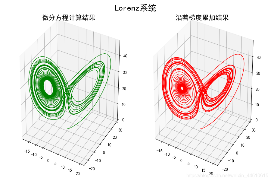
    plt.title('微分方程计算结果', fontsize=16)

    s = lorenz_trajectory(s0, 40000)
    plt.subplot(122, projection='3d')
    plt.plot(s[:, 0], s[:, 1], s[:, 2], c='r', lw=1)
    plt.title('沿着梯度累加结果', fontsize=16)

    plt.tight_layout(1, rect=(0,0,1,0.98))
    plt.suptitle('Lorenz系统', fontsize=20)
    plt.show()

    # Figure 2
    ax = Axes3D(plt.figure(figsize=(6, 6)))
    s0 = (0., 1., 0.)
    s1 = lorenz_trajectory(s0, 50000)
    s0 = (0., 1.0001, 0.)
    s2 = lorenz_trajectory(s0, 50000)
    # 曲线
    ax.plot(s1[:, 0], s1[:, 1], s1[:, 2], c='g', lw=0.4)
    ax.plot(s2[:, 0], s2[:, 1], s2[:, 2], c='r', lw=0.4)
    # 起点
    ax.scatter(s1[0, 0], s1[0, 1], s1[0, 2], c='g', s=50, alpha=0.5)
    ax.scatter(s2[0, 0], s2[0, 1], s2[0, 2], c='r', s=50, alpha=0.5)
    # 终点
    ax.scatter(s1[-1, 0], s1[-1, 1], s1[-1, 2], c='g', s=100)
    ax.scatter(s2[-1, 0], s2[-1, 1], s2[-1, 2], c='r', s=100)
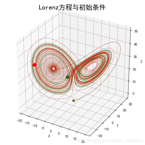
    ax.set_title('Lorenz方程与初始条件', fontsize=20)
    ax.set_xlabel('X')
    ax.set_ylabel('Y')
    ax.set_zlabel('Z')
    plt.show()