信用行为评分卡模型分析

这是一个kaggle上关于信用行为评分卡的项目，下面是我对该项目的分析过程

项目地址：https://www.kaggle.com/c/GiveMeSomeCredit/overview

数据地址：https://www.kaggle.com/c/GiveMeSomeCredit/data

1·首先对评分卡模型的定义如下

2·在kaggle上的项目说明文档如下表

数据分析流程：
1，数据获取
2，数据预处理（空值，异常值处理）
3，对数据进行分箱，woe编码，建模预估
4，评估模型的区分能力、预测能力、稳定性，并形成模型评估报告
5，将Logistic模型转换为标准评分

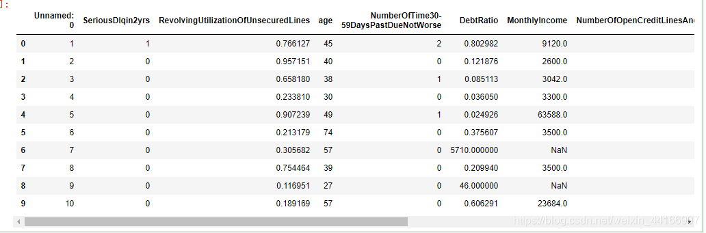
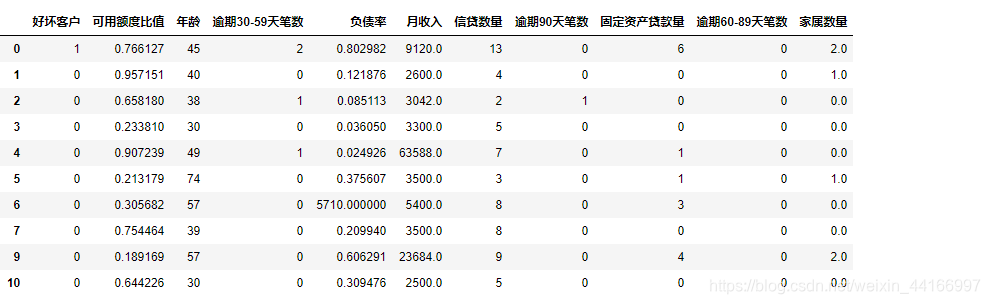
#读取数据
data = pd.read_csv(‘cs-training.csv’)
data.head(10)

#读取数据
data = pd.read_csv('cs-training.csv')
data.head(10)

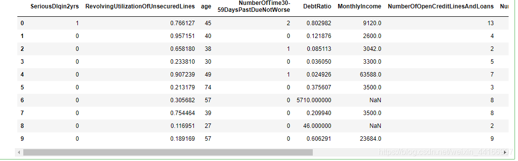
#删除与索引重复的Unnamed: 0列
data = data.drop('Unnamed: 0',axis=1)
data.head(10)

states={'SeriousDlqin2yrs':'好坏客户',
        'RevolvingUtilizationOfUnsecuredLines':'可用额度比值',
        'age':'年龄',
        'NumberOfTime30-59DaysPastDueNotWorse':'逾期30-59天笔数',
        'DebtRatio':'负债率',
        'MonthlyIncome':'月收入',
        'NumberOfOpenCreditLinesAndLoans':'信贷数量',
        'NumberOfTimes90DaysLate':'逾期90天笔数',
        'NumberRealEstateLoansOrLines':'固定资产贷款量',
        'NumberOfTime60-89DaysPastDueNotWorse':'逾期60-89天笔数',
        'NumberOfDependents':'家属数量'}
data.rename(columns=states,inplace=True)
data.head()    #修改英文字段名为中文字段名

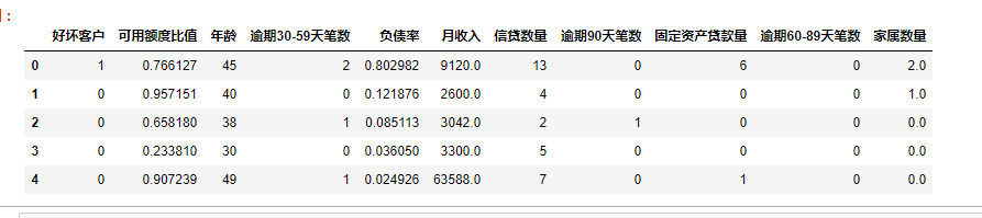
注意：这里 坏客户是1，好客户对应0，

一，数据预处理

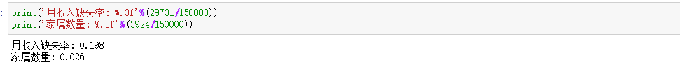
1,缺失值处理

#查看空值数量
data.isnull().sum()

#方法一缺失值处理
# 比较MonthlyIncome的中位数，平均数，众数，由于众数与中位数比较相近，故选择中位数作为空值填充值
# 对于NumberOfDependents ，因为缺失数据比例较少，所以直接舍弃这些数据
data1 = data.fillna({'月收入':5400})
data1=data1.dropna()
data1.head(10)

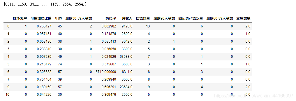
# 方法二通过随机森林填充空缺值
from sklearn.ensemble import RandomForestRegressor
# 定义方法
def set_missing(data):
    # 这里是对 '月收入' 这列的空值进行填充，故取值时不使用 '家属数量' 列的数据（因为有空缺值）
    # 把已有的数值型特征取出来
    process_data = data.iloc[:,[5,0,1,2,3,4,6,7,8,9]]
    # 分成已知该特征和未知该特征两部分
    known = process_data[process_data['月收入'].notnull()].values
    unknown = process_data[process_data['月收入'].isnull()].values
    # X为特征属性值
    x = known[:, 1:]
    # y为结果标签值
    y = known[:, 0]
    # fit到RandomForestRegressor之中
    rfr = RandomForestRegressor(random_state=0, n_estimators=200,max_depth=3,n_jobs=-1)
    rfr.fit(x,y)
    # 用得到的模型进行未知特征值预测
    predicted = rfr.predict(unknown[:, 1:]).round(0)
    print(predicted)
    # 用得到的预测结果填补原缺失数据
    data.loc[(data['月收入'].isnull()), '月收入'] = predicted
    
    #对于  '家属数量' ，因为缺失数据比例较少，所以直接直接舍弃这些数据
    data=data.dropna()
    return data
    
data2 = data.copy()
data2 = set_missing(data2)
data2.head(10)

2,异常值处理

from pylab import mpl    #用户设置字体
mpl.rcParams['font.sans-serif'] = ['SimHei']
x1=data2['可用额度比值']
x2=data2['负债率']
x3=data2["年龄"]
x4=data2["逾期30-59天笔数"]
x5=data2["逾期60-89天笔数"]
x6=data2["逾期90天笔数"]
x7=data2["信贷数量"]
x8=data2["固定资产贷款量"]
fig=plt.figure(figsize=(20,15))
ax1=fig.add_subplot(221)
ax2=fig.add_subplot(222)
ax3=fig.add_subplot(223)
ax4=fig.add_subplot(224)
ax1.boxplot([x1,x2])
ax1.set_xticklabels(["可用额度比值","负债率"], fontsize=20)
ax2.boxplot(x3)
ax2.set_xticklabels("年龄", fontsize=20)
ax3.boxplot([x4,x5,x6])
ax3.set_xticklabels(["逾期30-59天笔数","逾期60-89天笔数","逾期90天笔数"], fontsize=20)
ax4.boxplot([x7,x8])
ax4.set_xticklabels(["信贷数量","固定资产贷款量"], fontsize=20)

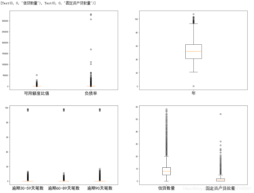
# 异常值处理消除不合逻辑的数据和超级离群的数据，可用额度比值应该小于1，年龄为0的是异常值，逾期天数笔数大于80的是超级离群数据，
# 固定资产贷款量大于50的是超级离群数据，将这些离群值过滤掉，筛选出剩余部分数据。
data2=data2[data2['可用额度比值']<1]
data2=data2[data2['年龄']>0]
data2=data2[data2['逾期30-59天笔数']<80]
data2=data2[data2['逾期60-89天笔数']<80]
data2=data2[data2['逾期90天笔数']<80]
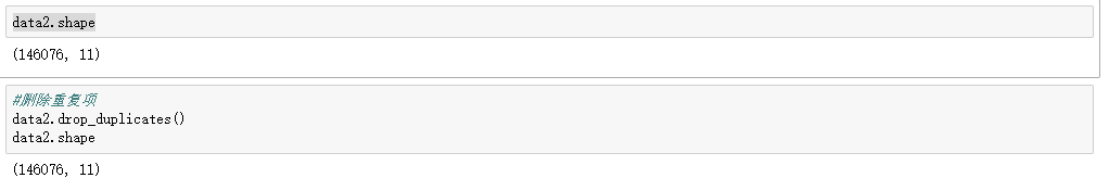
data2=data2[data2['固定资产贷款量']<50]
data2.shape

二，变量的相关性分析

1，单变量分析

2，多变量分析

相关性分析在整个流程当中对数据的变动不大，主要起到了一种催化的作用，作为一种“启动”开展后续工作，可以更好的了解到数据之间的一些联系和变化规律。同时在多变量分析中通过相关性也可以过滤掉一部分变量。所以此处不做详细探究。

三，特征选择

对数据进行分箱

pinf = float('inf')#正无穷大
ninf = float('-inf')#负无穷大
# 连续变量离散化
cutx3 = [ninf, 0, 1, 3, 5, pinf]
cutx6 = [ninf, 1, 2, 3, 5, pinf]
cutx7 = [ninf, 0, 1, 3, 5, pinf]
cutx8 = [ninf, 0,1,2, 3, pinf]
cutx9 = [ninf, 0, 1, 3, pinf]
cutx10 = [ninf, 0, 1, 2, 3, 5, pinf]

cut3=pd.cut(data2["逾期30-59天笔数"],cutx3,labels=False)
cut6=pd.cut(data2["信贷数量"],cutx6,labels=False)
cut7=pd.cut(data2["逾期90天笔数"],cutx7,labels=False)
cut8=pd.cut(data2["固定资产贷款量"],cutx8,labels=False)
cut9=pd.cut(data2["逾期60-89天笔数"],cutx9,labels=False)
cut10=pd.cut(data2["家属数量"],cutx10,labels=False)

#对数据进行等频分箱
cut1=pd.qcut(data2["可用额度比值"],4,labels=False)
cut2=pd.qcut(data2["年龄"],8,labels=False)
cut4=pd.qcut(data2["负债率"],3,labels=False)
cut5=pd.qcut(data2["月收入"],3,labels=False)

WOE值计算

rate=data2["好坏客户"].sum()/(data2["好坏客户"].count()-data2["好坏客户"].sum())
def get_woe_data(cut):
    grouped=data2["好坏客户"].groupby(cut,as_index = True).value_counts()
    woe=np.log(grouped.unstack().iloc[:,1]/grouped.unstack().iloc[:,0]/rate)
    return woe

cut1_woe=get_woe_data(cut1)
cut2_woe=get_woe_data(cut2)
cut3_woe=get_woe_data(cut3)
cut4_woe=get_woe_data(cut4)
cut5_woe=get_woe_data(cut5)
cut6_woe=get_woe_data(cut6)
cut7_woe=get_woe_data(cut7)
cut8_woe=get_woe_data(cut8)
cut9_woe=get_woe_data(cut9)
cut10_woe=get_woe_data(cut10)

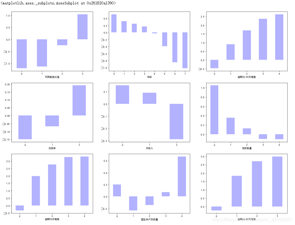
#抽选几个变量查看woe来分析分箱是否合理
fig=plt.figure(figsize=(20,15))
ax1=fig.add_subplot(331)
ax2=fig.add_subplot(332)
ax3=fig.add_subplot(333)
ax4=fig.add_subplot(334)
ax5=fig.add_subplot(335)
ax6=fig.add_subplot(336)
ax7=fig.add_subplot(337)
ax8=fig.add_subplot(338)
ax9=fig.add_subplot(339)
cut1_woe.plot.bar(ax=ax1,color='b',alpha=0.3,rot=0)
cut2_woe.plot.bar(ax=ax2,color='b',alpha=0.3,rot=0)
cut3_woe.plot.bar(ax=ax3,color='b',alpha=0.3,rot=0)
cut4_woe.plot.bar(ax=ax4,color='b',alpha=0.3,rot=0)
cut5_woe.plot.bar(ax=ax5,color='b',alpha=0.3,rot=0)
cut6_woe.plot.bar(ax=ax6,color='b',alpha=0.3,rot=0)
cut7_woe.plot.bar(ax=ax7,color='b',alpha=0.3,rot=0)
cut8_woe.plot.bar(ax=ax8,color='b',alpha=0.3,rot=0)
cut9_woe.plot.bar(ax=ax9,color='b',alpha=0.3,rot=0)

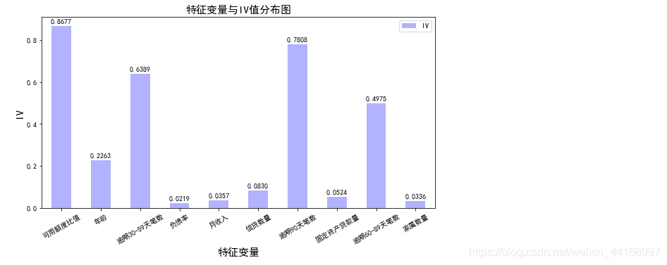
计算iv值

def get_IV_data(cut,cut_woe):
    grouped=data2["好坏客户"].groupby(cut,as_index = True).value_counts()
    cut_IV=((grouped.unstack().iloc[:,1]/data2["好坏客户"].sum()-grouped.unstack().iloc[:,0]/(data2["好坏客户"].count()-data2["好坏客户"].sum()))*cut_woe).sum()    
    return cut_IV
#计算各分组的IV值
cut1_IV=get_IV_data(cut1,cut1_woe)
cut2_IV=get_IV_data(cut2,cut2_woe)
cut3_IV=get_IV_data(cut3,cut3_woe)
cut4_IV=get_IV_data(cut4,cut4_woe)
cut5_IV=get_IV_data(cut5,cut5_woe)
cut6_IV=get_IV_data(cut6,cut6_woe)
cut7_IV=get_IV_data(cut7,cut7_woe)
cut8_IV=get_IV_data(cut8,cut8_woe)
cut9_IV=get_IV_data(cut9,cut9_woe)
cut10_IV=get_IV_data(cut10,cut10_woe)

ivlist = [cut1_IV,cut2_IV,cut3_IV,cut4_IV,cut5_IV,cut6_IV,cut7_IV,cut8_IV,cut9_IV,cut10_IV]
index=['可用额度比值','年龄','逾期30-59天笔数','负债率','月收入','信贷数量','逾期90天笔数','固定资产贷款量','逾期60-89天笔数','家属数量']
IV=pd.DataFrame(ivlist,index=index,columns=['IV'])
iv=IV.plot.bar(color='b',alpha=0.3,rot=30,figsize=(10,5),fontsize=(10))
iv.set_title('特征变量与IV值分布图',fontsize=(15))
iv.set_xlabel('特征变量',fontsize=(15))
iv.set_ylabel('IV',fontsize=(15))
x = np.arange(len(index))
for a, b in zip(x, ivlist):
    plt.text(a, b+0.01, '%.4f' % b, ha='center', va='bottom', fontsize=10)

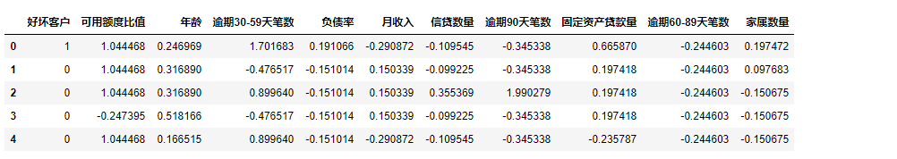
WOE值替换

woe_data=pd.DataFrame()   #新建df_new存放woe转换后的数据
def replace_data(cut,cut_woe):
    a=[]
    for i in cut.unique():
        a.append(i)
        a.sort()
    for m in range(len(a)):
        cut.replace(a[m],cut_woe.values[m],inplace=True)
    return cut
woe_data["好坏客户"]=data2["好坏客户"]
woe_data["可用额度比值"]=replace_data(cut1,cut1_woe)
woe_data["年龄"]=replace_data(cut2,cut2_woe)
woe_data["逾期30-59天笔数"]=replace_data(cut3,cut3_woe)
woe_data["负债率"]=replace_data(cut4,cut4_woe)
woe_data["月收入"]=replace_data(cut5,cut5_woe)
woe_data["信贷数量"]=replace_data(cut6,cut6_woe)
woe_data["逾期90天笔数"]=replace_data(cut7,cut7_woe)
woe_data["固定资产贷款量"]=replace_data(cut8,cut8_woe)
woe_data["逾期60-89天笔数"]=replace_data(cut9,cut9_woe)
woe_data["家属数量"]=replace_data(cut10,cut10_woe)
woe_data.head()

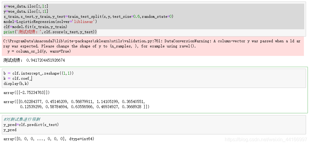
四，进行建模训练

x=woe_data.iloc[:,1:]
y=woe_data.iloc[:,:1]
x_train,x_test,y_train,y_test=train_test_split(x,y,test_size=0.6,random_state=0)
model=LogisticRegression(solver='liblinear')
clf=model.fit(x_train,y_train)
print('测试成绩：',clf.score(x_test,y_test))

b = clf.intercept_.reshape((1,1))
k = clf.coef_
display(b,k)

五，模型评估

# 模型评估主要看AUC和K-S值
fpr, tpr, threshold = roc_curve(y_test, y_pred)
roc_auc = auc(fpr, tpr)
plt.plot(fpr, tpr, color='darkorange',label='ROC curve (area = %0.2f)' % roc_auc)
plt.plot([0, 1], [0, 1], color='navy',  linestyle='--')
plt.xlim([0.0, 1.0])
plt.ylim([0.0, 1.0])
plt.xlabel('False Positive Rate')
plt.ylabel('True Positive Rate')
plt.title('ROC_curve')
plt.legend(loc="lower right")
plt.show()

fig, ax = plt.subplots()
ax.plot(1 - threshold, tpr, label='tpr') # ks曲线要按照预测概率降序排列，所以需要1-threshold镜像
ax.plot(1 - threshold, fpr, label='fpr')
ax.plot(1 - threshold, tpr-fpr,label='KS')
plt.xlabel('score')
plt.title('KS Curve')
plt.ylim([0.0, 1.0])
plt.figure(figsize=(20,20))
legend = ax.legend(loc='upper left')
plt.show()

六，模型结果转评分

#计算各特征的得分
factor = 20 / np.log(2)
offset = 600 - 20 * np.log(20) / np.log(2)
def get_score(coe,woe,factor):
    scores=[]
    for w in woe:
        score=round(coe*w*factor,0)
        scores.append(score)
    return scores
x1 = get_score(k[0][0], cut1_woe, factor)
x2 = get_score(k[0][1], cut2_woe, factor)
x3 = get_score(k[0][2], cut3_woe, factor)
x4 = get_score(k[0][3], cut4_woe, factor)
x5 = get_score(k[0][4], cut5_woe, factor)
x6 = get_score(k[0][5], cut6_woe, factor)
x7 = get_score(k[0][6], cut7_woe, factor)
x8 = get_score(k[0][7], cut8_woe, factor)
x9 = get_score(k[0][8], cut9_woe, factor)
x10 = get_score(k[0][9], cut10_woe, factor)
print("可用额度比值对应的分数:{}".format(x1))
print("年龄对应的分数:{}".format(x2))
print("逾期30-59天笔数对应的分数:{}".format(x3))
print("负债率对应的分数:{}".format(x4))
print("月收入对应的分数:{}".format(x5))
print("信贷数量对应的分数:{}".format(x6))
print("逾期90天笔数对应的分数:{}".format(x7))
print("固定资产贷款量对应的分数:{}".format(x8))
print("逾期60-89天笔数对应的分数:{}".format(x9))
print("家属数量对应的分数:{}".format(x10))

#根据变量计算分数
def compute_score(series,cut,score):
    for i,j in zip(cut.values,score):
        series.replace({i:j},inplace=True)
    return series

ScoreDat =pd.DataFrame()
ScoreDat['x1'] = compute_score(x_test['可用额度比值'], cut1_woe, x1)
ScoreDat['x2'] = compute_score(x_test['年龄'], cut2_woe, x2)
ScoreDat['x3'] = compute_score(x_test['逾期30-59天笔数'], cut3_woe, x3)
ScoreDat['x4'] = compute_score(x_test['负债率'], cut4_woe, x4)
ScoreDat['x5'] = compute_score(x_test['月收入'], cut5_woe, x5)
ScoreDat['x6'] = compute_score(x_test['信贷数量'], cut6_woe, x6)
ScoreDat['x7'] = compute_score(x_test['逾期90天笔数'], cut7_woe, x7)
ScoreDat['x8'] = compute_score(x_test['固定资产贷款量'], cut8_woe, x8)
ScoreDat['x9'] = compute_score(x_test['逾期60-89天笔数'], cut9_woe, x9)
ScoreDat['x10'] = compute_score(x_test['家属数量'], cut10_woe, x10)
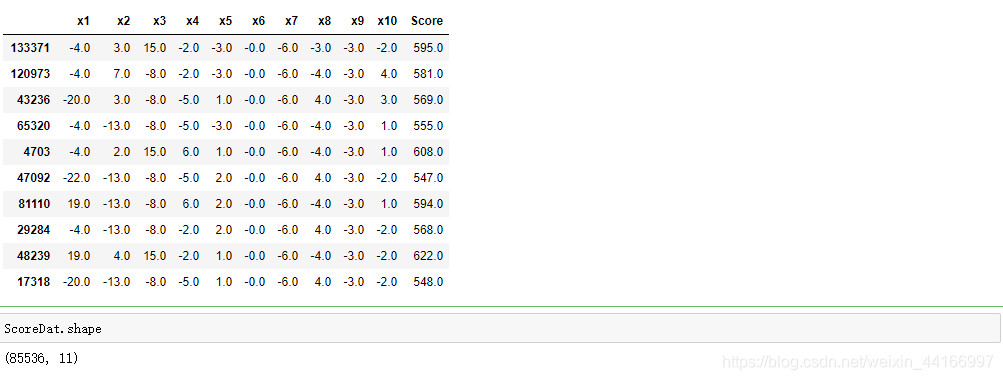
ScoreDat['Score'] = ScoreDat['x1'] + ScoreDat['x2'] + ScoreDat['x3'] +ScoreDat['x4'] +ScoreDat['x5']+ ScoreDat['x6']+ScoreDat['x7'] +ScoreDat['x8']+ ScoreDat['x9'] +ScoreDat['x10'] + 600
ScoreDat.head(10)

#重排索引
ScoreDat.reset_index(drop=True,inplace=True)
ScoreDat.head()