1. 前言

《MATLAB 神经网络43个案例分析》是MATLAB技术论坛（www.matlabsky.com）策划，由王小川老师主导，2013年北京航空航天大学出版社出版的关于MATLAB为工具的一本MATLAB实例教学书籍，是在《MATLAB神经网络30个案例分析》的基础上修改、补充而成的，秉承着“理论讲解—案例分析—应用扩展”这一特色，帮助读者更加直观、生动地学习神经网络。

《MATLAB神经网络43个案例分析》共有43章，内容涵盖常见的神经网络（BP、RBF、SOM、Hopfield、Elman、LVQ、Kohonen、GRNN、NARX等）以及相关智能算法（SVM、决策树、随机森林、极限学习机等）。同时，部分章节也涉及了常见的优化算法（遗传算法、蚁群算法等）与神经网络的结合问题。此外，《MATLAB神经网络43个案例分析》还介绍了MATLAB R2012b中神经网络工具箱的新增功能与特性，如神经网络并行计算、定制神经网络、神经网络高效编程等。

近年来随着人工智能研究的兴起，神经网络这个相关方向也迎来了又一阵研究热潮，由于其在信号处理领域中的不俗表现，神经网络方法也在不断深入应用到语音和图像方向的各种应用当中，本文结合书中案例，对其进行仿真实现，也算是进行一次重新学习，希望可以温故知新，加强并提升自己对神经网络这一方法在各领域中应用的理解与实践。自己正好在多抓鱼上入手了这本书，下面开始进行仿真示例，主要以介绍各章节中源码应用示例为主，本文主要基于MATLAB2015b(32位)平台仿真实现，这是本书第八章GRNN网络的预测实例，话不多说，开始！

2. MATLAB 仿真示例一

打开MATLAB，点击“主页”，点击“打开”，找到示例文件
在这里插入图片描述
选中chapter8_1.m，点击“打开”

chapter8_1.m源码如下：

%%%%%%%%%%%%%%%%%%%%%%%%%%%%%%%%%%%%%%%%%%%%%%%%%%%%
%功能：GRNN的数据预测—基于广义回归神经网络的货运量预测
%环境：Win7，Matlab2015b
%Modi: C.S
%时间：2022-06-09
%%%%%%%%%%%%%%%%%%%%%%%%%%%%%%%%%%%%%%%%%%%%%%%%%%%%

%% Matlab神经网络43个案例分析

% GRNN的数据预测—基于广义回归神经网络的货运量预测
% by 王小川(@王小川_matlab)
% http://www.matlabsky.com
% Email:sina363@163.com
% http://weibo.com/hgsz2003
 
%% 清空环境变量
clc;
clear all
close all
nntwarn off;
tic
%% 载入数据
load data;
% 载入数据并将数据分成训练和预测两类
p_train=p(1:12,:);
t_train=t(1:12,:);
p_test=p(13,:);
t_test=t(13,:);
%% 交叉验证
desired_spread=[];
mse_max=10e20;
desired_input=[];
desired_output=[];
result_perfp=[];
indices = crossvalind('Kfold',length(p_train),4);
h=waitbar(0,'正在寻找最优化参数....');
k=1;
for i = 1:4
    perfp=[];
    disp(['以下为第',num2str(i),'次交叉验证结果'])
    test = (indices == i); train = ~test;
    p_cv_train=p_train(train,:);
    t_cv_train=t_train(train,:);
    p_cv_test=p_train(test,:);
    t_cv_test=t_train(test,:);
    p_cv_train=p_cv_train';
    t_cv_train=t_cv_train';
    p_cv_test= p_cv_test';
    t_cv_test= t_cv_test';
    [p_cv_train,minp,maxp,t_cv_train,mint,maxt]=premnmx(p_cv_train,t_cv_train);
    p_cv_test=tramnmx(p_cv_test,minp,maxp);
    for spread=0.1:0.1:2;
        net=newgrnn(p_cv_train,t_cv_train,spread);
        waitbar(k/80,h);
        disp(['当前spread值为', num2str(spread)]);
        test_Out=sim(net,p_cv_test);
        test_Out=postmnmx(test_Out,mint,maxt);
        error=t_cv_test-test_Out;
        disp(['当前网络的mse为',num2str(mse(error))])
        perfp=[perfp mse(error)];
        if mse(error)<mse_max
            mse_max=mse(error);
            desired_spread=spread;
            desired_input=p_cv_train;
            desired_output=t_cv_train;
        end
        k=k+1;
    end
    result_perfp(i,:)=perfp;
end;
close(h)
disp(['最佳spread值为',num2str(desired_spread)])
disp(['此时最佳输入值为'])
desired_input
disp(['此时最佳输出值为'])
desired_output
%% 采用最佳方法建立GRNN网络
net=newgrnn(desired_input,desired_output,desired_spread);
p_test=p_test';
p_test=tramnmx(p_test,minp,maxp);
grnn_prediction_result=sim(net,p_test);
grnn_prediction_result=postmnmx(grnn_prediction_result,mint,maxt);
grnn_error=t_test-grnn_prediction_result';
disp(['GRNN神经网络三项流量预测的误差为',num2str(abs(grnn_error))])
save best desired_input desired_output p_test t_test grnn_error mint maxt
toc

添加完毕，点击“运行”，开始仿真，输出仿真结果如下：

以下为第1次交叉验证结果
当前spread值为0.1
当前网络的mse为472661451.4318
当前spread值为0.2
当前网络的mse为431495393.7817
当前spread值为0.3
当前网络的mse为382468361.129
当前spread值为0.4
当前网络的mse为280914533.8622
当前spread值为0.5
当前网络的mse为212911900.1912
当前spread值为0.6
当前网络的mse为190718117.4076
当前spread值为0.7
当前网络的mse为185701936.8467
当前spread值为0.8
当前网络的mse为182815185.6709
当前spread值为0.9
当前网络的mse为179262063.2524
当前spread值为1
当前网络的mse为177028588.7682
当前spread值为1.1
当前网络的mse为178057284.4181
当前spread值为1.2
当前网络的mse为183091720.765
当前spread值为1.3
当前网络的mse为192096590.0633
当前spread值为1.4
当前网络的mse为204774132.931
当前spread值为1.5
当前网络的mse为220820271.3226
当前spread值为1.6
当前网络的mse为239984981.0069
当前spread值为1.7
当前网络的mse为262048640.2103
当前spread值为1.8
当前网络的mse为286783239.802
当前spread值为1.9
当前网络的mse为313926435.5194
当前spread值为2
当前网络的mse为343173556.2188
以下为第2次交叉验证结果
当前spread值为0.1
当前网络的mse为139271525.2083
当前spread值为0.2
当前网络的mse为80576363.9605
当前spread值为0.3
当前网络的mse为68025918.339
当前spread值为0.4
当前网络的mse为65711476.2141
当前spread值为0.5
当前网络的mse为67990375.0282
当前spread值为0.6
当前网络的mse为75213536.3146
当前spread值为0.7
当前网络的mse为85895033.7216
当前spread值为0.8
当前网络的mse为98031033.349
当前spread值为0.9
当前网络的mse为110783983.0205
当前spread值为1
当前网络的mse为124594358.424
当前spread值为1.1
当前网络的mse为140572319.5568
当前spread值为1.2
当前网络的mse为159946177.7931
当前spread值为1.3
当前网络的mse为183760280.5868
当前spread值为1.4
当前网络的mse为212758877.6147
当前spread值为1.5
当前网络的mse为247371509.8989
当前spread值为1.6
当前网络的mse为287745538.6363
当前spread值为1.7
当前网络的mse为333795159.1579
当前spread值为1.8
当前网络的mse为385250286.5875
当前spread值为1.9
当前网络的mse为441697951.9133
当前spread值为2
当前网络的mse为502615420.243
以下为第3次交叉验证结果
当前spread值为0.1
当前网络的mse为141150162.9514
当前spread值为0.2
当前网络的mse为128111068.5282
当前spread值为0.3
当前网络的mse为83744006.0734
当前spread值为0.4
当前网络的mse为67423942.7694
当前spread值为0.5
当前网络的mse为61372652.5932
当前spread值为0.6
当前网络的mse为51578033.4398
当前spread值为0.7
当前网络的mse为39870045.1462
当前spread值为0.8
当前网络的mse为30432282.7062
当前spread值为0.9
当前网络的mse为24696141.3181
当前spread值为1
当前网络的mse为22254241.0689
当前spread值为1.1
当前网络的mse为22274220.4151
当前spread值为1.2
当前网络的mse为24105743.8546
当前spread值为1.3
当前网络的mse为27386943.3443
当前spread值为1.4
当前网络的mse为31986233.7649
当前spread值为1.5
当前网络的mse为37924227.0431
当前spread值为1.6
当前网络的mse为45311202.6528
当前spread值为1.7
当前网络的mse为54298847.1454
当前spread值为1.8
当前网络的mse为65040087.8156
当前spread值为1.9
当前网络的mse为77655044.589
当前spread值为2
当前网络的mse为92205035.9882
以下为第4次交叉验证结果
当前spread值为0.1
当前网络的mse为126953769.5897
当前spread值为0.2
当前网络的mse为73390966.1325
当前spread值为0.3
当前网络的mse为30326167.3505
当前spread值为0.4
当前网络的mse为18454401.3125
当前spread值为0.5
当前网络的mse为14611371.7325
当前spread值为0.6
当前网络的mse为13137052.7123
当前spread值为0.7
当前网络的mse为13357597.5513
当前spread值为0.8
当前网络的mse为14909865.4094
当前spread值为0.9
当前网络的mse为17573134.5699
当前spread值为1
当前网络的mse为21481700.3926
当前spread值为1.1
当前网络的mse为27032218.047
当前spread值为1.2
当前网络的mse为34721466.9003
当前spread值为1.3
当前网络的mse为45037209.6584
当前spread值为1.4
当前网络的mse为58393976.2438
当前spread值为1.5
当前网络的mse为75097536.6486
当前spread值为1.6
当前网络的mse为95330559.7536
当前spread值为1.7
当前网络的mse为119152174.2514
当前spread值为1.8
当前网络的mse为146504792.3109
当前spread值为1.9
当前网络的mse为177224697.3974
当前spread值为2
当前网络的mse为211055741.5274
最佳spread值为0.6
此时最佳输入值为

desired_input =

   -1.0000   -0.9578   -0.7570   -0.4706   -0.2682   -0.0351    0.3968    0.6723    1.0000
   -0.9552   -1.0000   -0.1293   -0.0073    0.2069    0.3416    0.6186    0.7838    1.0000
   -1.0000   -1.0000   -0.4969   -0.4969    0.1950    0.3333    0.6478    0.6604    1.0000
   -1.0000   -1.0000   -0.0769    0.5385    0.2308    0.3846    0.6923    0.6923    1.0000
   -1.0000   -0.9749   -0.8934   -0.7555   -0.5737   -0.3103    0.2602    0.5674    1.0000
   -1.0000   -0.7391   -0.7391   -0.3043   -0.1304   -0.0435    0.3043    0.5652    1.0000
   -1.0000   -0.9945   -0.9852   -0.9852   -0.5220   -0.2781    0.2302    0.5418    1.0000
   -1.0000   -0.7677   -0.6639   -0.7291   -0.5720   -0.4229    0.0881    0.3674    1.0000

此时最佳输出值为

desired_output =

   -1.0000   -0.9931   -0.9770   -0.7068   -0.4453   -0.2420    0.2887    0.5410    1.0000
   -1.0000   -0.9401   -0.8046   -0.5911   -0.3532   -0.1924    0.2360    0.4292    1.0000
   -1.0000   -0.9512   -0.7602   -0.5070   -0.2167   -0.0244    0.2688    0.4823    1.0000

GRNN神经网络三项流量预测的误差为10535.1574      2208.87442      14835.2722
时间已过 7.248012 秒。

3. MATLAB 仿真示例二

双击当前文件夹视图中的chapter8_2.m，打开chapter8_2.m源码如下：

%%%%%%%%%%%%%%%%%%%%%%%%%%%%%%%%%%%%%%%%%%%%%%%%%%%%
%功能：GRNN的数据预测—基于广义回归神经网络的货运量预测
%环境：Win7，Matlab2015b
%Modi: C.S
%时间：2022-06-09
%%%%%%%%%%%%%%%%%%%%%%%%%%%%%%%%%%%%%%%%%%%%%%%%%%%%

%% Matlab神经网络43个案例分析

% GRNN的数据预测—基于广义回归神经网络的货运量预测
% by 王小川(@王小川_matlab)
% http://www.matlabsky.com
% Email:sina363@163.com
% http://weibo.com/hgsz2003
 
%% 以下程序为案例扩展里的GRNN和BP比较 需要load chapter8.1的相关数据
clear all
tic
load best
n=13
p=desired_input
t=desired_output
net_bp=newff(minmax(p),[n,3],{
    
    'tansig','purelin'},'trainlm');
% 训练网络
net.trainParam.show=50;
net.trainParam.epochs=2000;
net.trainParam.goal=1e-3;
%调用TRAINLM算法训练BP网络
net_bp=train(net_bp,p,t);
bp_prediction_result=sim(net_bp,p_test);
bp_prediction_result=postmnmx(bp_prediction_result,mint,maxt);
bp_error=t_test-bp_prediction_result';
disp(['BP神经网络三项流量预测的误差为',num2str(abs(bp_error))])
toc

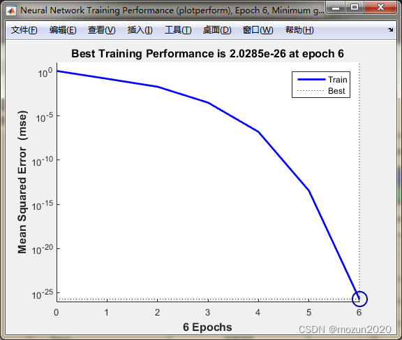
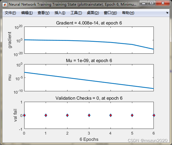
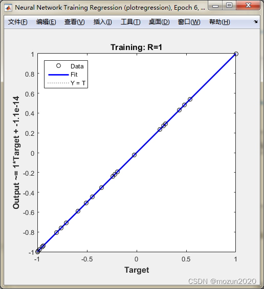
点击“运行”，开始仿真，输出仿真结果如下：

         See help for NEWFF to update calls to the new argument list.
 
BP神经网络三项流量预测的误差为55999.9467      23112.3167      21737.7695
时间已过 2.467178 秒。

在这里插入图片描述
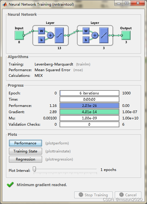
依次点击Performance，Training State，Regression可分别得到如下对应图示。

4. 小结

GRNN网络，即广义回归神经网络，它是径向基神经网络的一种，GRNN具有很强的非线性映射能力和学习速度，比RBF具有更强的优势，网络最后普收敛于样本量集聚较多的优化回归，样本数据少时，预测效果很好，还可以处理不稳定数据。虽然GRNN看起来没有径向基精准，但实际在分类和拟合上，特别是数据精准度比较差的时候有着很大的优势。对本章内容感兴趣或者想充分学习了解的，建议去研习书中第八章节的内容。后期会对其中一些知识点在自己理解的基础上进行补充，欢迎大家一起学习交流。

《MATLAB 神经网络43个案例分析》：第8章 GRNN网络的预测----基于广义回归神经网络的货运量预测

《MATLAB 神经网络43个案例分析》：第8章 GRNN网络的预测----基于广义回归神经网络的货运量预测

1. 前言

2. MATLAB 仿真示例一

3. MATLAB 仿真示例二

4. 小结

猜你喜欢