AIGC-从代码角度去理解DDPM(扩散模型)

最近准备要学习一下AIGC，因此需要从一些基本网络开始了解，比如DDPM，本篇文章会从代码解析角度来供大家学习了解。DDPM(Denoising Diffusion Probabilistic Models) 是一种扩散模型。

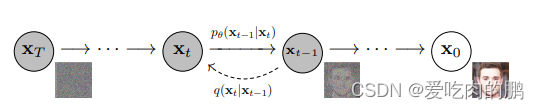
扩散模型包含两个主要的过程：加噪过程和去噪过程。对应到上述图中，从x0到xt是加噪的过程，从xt到x0是去噪的过程。

前向加噪过程和反向去噪过程都是马尔可夫链，全过程大约需要1000步。

前向的加噪过程是对输入数据不断的加噪声(高斯噪声)。

反向去噪过程是对从标准高斯分布中逐步地得到一个个噪声样本，最终得到生成的样本的数据。

其中加噪过程的公式为：

$x_{t}=\sqrt{\alpha_{t}}x_{t-1}+\sqrt{1-\alpha _{t}}z_{1}$

这里的 $\sqrt{\alpha_{t}}$ 是提前设置好的超参数，称为Noise schedule,通常是小于1的值，取值为0.9999到0.998。【上式表示了 $x_{t}$ 是如何从 $x_{t-1}$ 推导出来】。

那么 $x_{t}$ 和 $x_{t-2}$ 的关系是什么呢？我们可以在往前推导一下（就是将 $x_{t-1}$ 展开）：

$x_{t}=\sqrt{\alpha _{t}}(\sqrt{\alpha_{t-1}}x_{t-2}+\sqrt{1-\alpha_{t-1}}z_{2})+\sqrt{1-\alpha_{t}}z_{1}$

其中每次加入的噪声都服从正态分布 $z_{1},z_{2}...\sim N(0,1)$ ,因此对上式整理一下可以得到：

$x_{t}=\sqrt{\alpha_{t}\alpha_{t-1}}x_{t-2}+\sqrt{1-\alpha_{t}\alpha_{t-1}}z_{2}$

那么我们是不是就找到了一定的规律，就可以得出 $x_{t}$ 和 $x_{0}$ 的关系式了：

$x_{t}=\sqrt{\overline{\alpha_{t}}}x_{x0}+\sqrt{1-\overline{\alpha_{t}}}z_{t}$

DDPM在代码中的定义如下：

代码采用的是Bubbliiing的代码。

net    = GaussianDiffusion(UNet(3, self.channel), self.input_shape, 3, betas=betas)

可以看到该扩散模型传入参数有UNet网络，input_shape为输入大小，3指的图像输入通道，betas为一个线性时间表，可用于生成噪声表(也就是文章最开始介绍的Noise schedule $\alpha _{t}$ )，其值在 schedule_low 和 schedule_high 之间，在总时间步数 num_timesteps (这里设置的是1000)内均匀分布。而betas定义如下(当然你可以可以用cosine生成，这里我只是用线性的举例子)：

betas = generate_linear_schedule(
                self.num_timesteps,
                self.schedule_low * 1000 / self.num_timesteps,
                self.schedule_high * 1000 / self.num_timesteps,
            )

训练forward函数部分

然后我们进入GaussianDiffusion的代码内部看一下各个组成部分。我们直接去看一下内部的forward函数，看看是如何处理图片的。

    def forward(self, x, y=None):
        b, c, h, w  = x.shape
        device      = x.device

        if h != self.img_size[0]:
            raise ValueError("image height does not match diffusion parameters")
        if w != self.img_size[0]:
            raise ValueError("image width does not match diffusion parameters")
        # 随机生成batch个范围在0~1000内的数
        t = torch.randint(0, self.num_timesteps, (b,), device=device)
        return self.get_losses(x, t, y)

可以看到在GaussianDiffusion的forward部分，x是输入的图片，然后里面有个t，表示随机生成范围在0~num_timesteps【时间步长】batch_size个数，或者可以理解为给每个batch(图片)随机打上时间戳。然后再一步一步深挖代码，进入get_losses函数。

get_losses部分

下面是get_losses代码，有三个输入，x,t,y。这里的x就是我们训练输入的图片，t就是上面随机生成的时间戳。

    def get_losses(self, x, t, y):
        # x, noise [batch_size, 3, 64, 64]
        noise           = torch.randn_like(x)  # 产生与输入图片shape一样的随机噪声(正态分布)

        perturbed_x     = self.perturb_x(x, t, noise)
        estimated_noise = self.model(perturbed_x, t, y)

        if self.loss_type == "l1":
            loss = F.l1_loss(estimated_noise, noise)
        elif self.loss_type == "l2":
            loss = F.mse_loss(estimated_noise, noise)
        return loss

在函数内部首先是创建了一个与输入图片大小的相同的符合正态分布的随机噪声noise，然后perturb_x函数是对输入图片在时间t上加入噪声进行加噪的扰动处理。

perturb_x函数部分

那么就看一下perturb_x中是如何给图片在时间t上加噪的(要保持头脑清醒，这些代码和套娃一样一层一层的)。

在该函数中有三个输入参数：x(输入图片)，t(时间序列)，noise(随机噪声)，函数最终返回的是经过加噪(扰动)后的图像，比如我现在输入一张图片，然后此时的t=323,那么就可以理解为在时间戳为323的时候为我的这张图加上噪声t，而这图就是对应于t时刻的输入Xt。sqrt_alphas_cumprod和sqrt_one_minus_alphas_cumprod 使用了这两个张量来控制输入图像x和噪声noise在时间维度上的混合比例。

    def perturb_x(self, x, t, noise):
        '''
        :param x:输入图像
        :param t: 每个图片不同的时间戳(范围在0~1000)
        :param noise: 与输入图片shape一样的正态分布随机噪声
        :return:经过扰动后的图像
        '''
        return (
            extract(self.sqrt_alphas_cumprod, t,  x.shape) * x +
            extract(self.sqrt_one_minus_alphas_cumprod, t, x.shape) * noise
        )

我们可以对perturb_x的过程进行可视化，比如我有下面一张未加噪声的原始图片：

通过perturb_x对x进行扰动加噪后的效果：

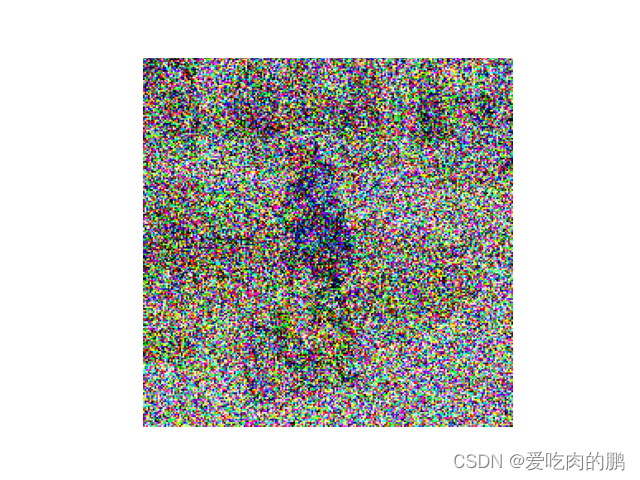
我们还可以控制噪声在图像上的扩散扰动效果：

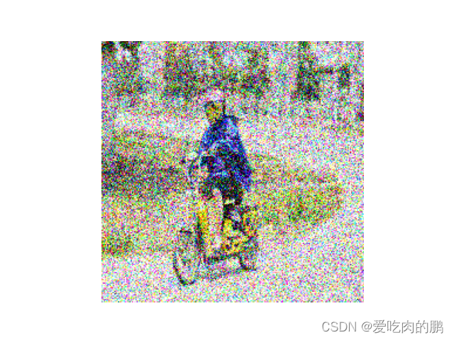
上面就是通过对时间t时刻对应的图片Xt加噪的处理过程了。会随着时间t的推移而变得越来越模糊。

然后再返回get_losses函数(代码如下)，perturbed_x就是我们加噪后的t时刻的图片Xt，然后这里的model就是我们的主干网络UNet网络(UNet网络部分我会单独拿出来)。那么可以总结一下get_losses的主要过程：

步骤1.通过perturb_x对输入图像进行时间域上的扰动，并与随机噪声 noise 混合，生成 perturbed_x 扰动后的图像；

步骤2.通过UNet网络对加噪后的图像进行预测，得到预测后的噪声信号estimated_noise。

步骤3.计算预测噪声estimated_noise和真实噪声noise的loss。

    def get_losses(self, x, t, y):
        # x, noise [batch_size, 3, 64, 64]
        noise           = torch.randn_like(x)  # 产生与输入图片shape一样的随机噪声(正态分布)

        perturbed_x     = self.perturb_x(x, t, noise)
        estimated_noise = self.model(perturbed_x, t, y)

        if self.loss_type == "l1":
            loss = F.l1_loss(estimated_noise, noise)
        elif self.loss_type == "l2":
            loss = F.mse_loss(estimated_noise, noise)
        return loss

也就是在训练阶段是计算的预测噪声和真实噪声的Loss关系。

预测阶段

    @torch.no_grad()
    def sample(self, batch_size, device, y=None, use_ema=True):
        if y is not None and batch_size != len(y):
            raise ValueError("sample batch size different from length of given y")

        x = torch.randn(batch_size, self.img_channels, *self.img_size, device=device)
        
        for t in tqdm(range(self.num_timesteps - 1, -1, -1), desc='remove noise....'):
            t_batch = torch.tensor([t], device=device).repeat(batch_size)
            x = self.remove_noise(x, t_batch, y, use_ema)

            if t > 0:
                x += extract(self.sigma, t_batch, x.shape) * torch.randn_like(x)
        
        return x.cpu().detach()

预测阶段即对输入的噪声(这里就不是输入的图像了)进行去噪处理，得到最终生成的图像。

输入一个正态分布噪声x，然后不断的去噪(Xt~X0的过程)。

网络模型结构

DDP是由Unet组成的，那就先看一下Unet中的组成。

class UNet(nn.Module):
    def __init__(
        self, img_channels, base_channels=128, channel_mults=(1, 2, 4, 8),
        num_res_blocks=3, time_emb_dim=128 * 4, time_emb_scale=1.0, num_classes=None, activation=SiLU(),
        dropout=0.1, attention_resolutions=(1,), norm="gn", num_groups=32, initial_pad=0,
    ):

time_mlp

self.time_mlp = nn.Sequential(
            PositionalEmbedding(base_channels, time_emb_scale),
            nn.Linear(base_channels, time_emb_dim),
            SiLU(),
            nn.Linear(time_emb_dim, time_emb_dim),
        ) if time_emb_dim is not None else None

time_mlp又由PositionalEmbedding层、Linear、SiLu、Linear组成。

PositionalEmbedding层

class PositionalEmbedding(nn.Module):
    def __init__(self, dim, scale=1.0):
        super().__init__()
        assert dim % 2 == 0
        self.dim = dim
        self.scale = scale

    def forward(self, x):
        device      = x.device
        half_dim    = self.dim // 2
        emb = math.log(10000) / half_dim
        emb = torch.exp(torch.arange(half_dim, device=device) * -emb)
        # x * self.scale和emb外积
        emb = torch.outer(x * self.scale, emb)
        emb = torch.cat((emb.sin(), emb.cos()), dim=-1)
        return emb

代码中forward中的x为time(时间轴)，并不是图像。

该函数主要是用来做位置编码的。而位置编码可以用正余弦来计算位置。所用到的公式为：

$PE_{pos,2i}=sin(pos/10000^{2i/d_{model}})$

$PE_{pos,2i+1}=cos(pos/10000^{2i/d_{model}})$

在位置编码公式中，pos 表示序列中的每个位置的索引。对于长度为 4 的序列 x，每个位置的索引从 0 到 3。在计算每个位置的位置编码向量时，我们会利用这个索引值进行计算。

具体来说，公式中的 pos 表示序列中的位置索引，在计算位置编码向量的过程中，会使用它来计算正弦和余弦的函数参数。

例如，在计算位置编码矩阵的第一个位置编码向量时，pos 的值为 0；在计算第二个位置编码向量时，pos 的值为 1，以此类推。

可以举个例子，比如我现在有个序列X,长度为4，位置编码的维度也设置为4.然后计算每个序列的位置信息(通过正余弦)

# 设置向量的长度和位置编码的维度
vector_length = 4
embedding_dim = 4

# 生成位置编码矩阵
pos_encoding = np.zeros((vector_length, embedding_dim))

for pos in range(vector_length):
    for i in range(embedding_dim):
        if i % 2 == 0:
            pos_encoding[pos, i] = np.sin(pos / (10000 ** (2 * i / embedding_dim)))
        else:
            pos_encoding[pos, i] = np.cos(pos / (10000 ** (2 * (i - 1) / embedding_dim)))

# 打印位置编码矩阵
print(pos_encoding)

得到的位置编码矩阵如下

[[ 0.00000000e+00 1.00000000e+00 0.00000000e+00 1.00000000e+00]
[ 8.41470985e-01 5.40302306e-01 9.99999998e-05 9.99999995e-01]
[ 9.09297427e-01 -4.16146837e-01 1.99999999e-04 9.99999980e-01]
[ 1.41120008e-01 -9.89992497e-01 2.99999995e-04 9.99999955e-01]]

其中，数组的每一行对应位置编码矩阵的一个位置，第一列表示正弦函数在该位置上的取值，第二列表示余弦函数在该位置上的取值，以此类推。

也就是说在该函数中，我们可以将输入信息的位置信息，通过sin和cos映射到高纬度空间中，得到位置特征。

ResidualBlock

class ResidualBlock(nn.Module):
    def __init__(
        self, in_channels, out_channels, dropout, time_emb_dim=None, num_classes=None, activation=SiLU(),
        norm="gn", num_groups=32, use_attention=False,
    ):
        super().__init__()

        self.activation = activation

        self.norm_1 = get_norm(norm, in_channels, num_groups)
        self.conv_1 = nn.Conv2d(in_channels, out_channels, 3, padding=1)

        self.norm_2 = get_norm(norm, out_channels, num_groups)
        self.conv_2 = nn.Sequential(
            nn.Dropout(p=dropout), 
            nn.Conv2d(out_channels, out_channels, 3, padding=1),
        )

        self.time_bias  = nn.Linear(time_emb_dim, out_channels) if time_emb_dim is not None else None
        self.class_bias = nn.Embedding(num_classes, out_channels) if num_classes is not None else None

        self.residual_connection    = nn.Conv2d(in_channels, out_channels, 1) if in_channels != out_channels else nn.Identity()
        self.attention              = nn.Identity() if not use_attention else AttentionBlock(out_channels, norm, num_groups)
    
    def forward(self, x, time_emb=None, y=None):
        out = self.activation(self.norm_1(x))
        # 第一个卷积
        out = self.conv_1(out)
        
        # 对时间time_emb做一个全连接，施加在通道上
        if self.time_bias is not None:
            if time_emb is None:
                raise ValueError("time conditioning was specified but time_emb is not passed")
            out += self.time_bias(self.activation(time_emb))[:, :, None, None]

        # 对种类y_emb做一个全连接，施加在通道上
        if self.class_bias is not None:
            if y is None:
                raise ValueError("class conditioning was specified but y is not passed")

            out += self.class_bias(y)[:, :, None, None]

        out = self.activation(self.norm_2(out))
        # 第二个卷积+残差边
        out = self.conv_2(out) + self.residual_connection(x)
        # 最后做个Attention
        out = self.attention(out)
        return out

。。。。暂未更新完