《------往期经典推荐------》
二、机器学习实战专栏【链接】,已更新31期,欢迎关注,持续更新中~~
三、深度学习【Pytorch】专栏【链接】
四、【Stable Diffusion绘画系列】专栏【链接】
五、YOLOv8改进专栏【链接】,持续更新中~~
六、YOLO性能对比专栏【链接】,持续更新中~
《------正文------》
论文地址:https://arxiv.org/abs/2309.03329
代码地址:https://github.com/UARK-AICV/MEGANet
摘要
本文提出了一种名为**多尺度边缘引导注意力网络(MEGANet)**的新方法,用于结肠镜图像中的息肉分割。息肉分割在结直肠癌的早期诊断中起着至关重要的作用,但由于背景复杂、息肉大小和形状多变以及边界模糊,分割任务面临诸多挑战。MEGANet通过结合经典的边缘检测技术和注意力机制,有效保留了高频信息(如边缘和边界),从而提高了分割精度。该方法在五个基准数据集上进行了广泛的实验,结果表明MEGANet在六种评估指标上均优于现有的最先进方法。
创新点
-
边缘引导注意力模块(EGA):MEGANet的核心创新是引入了EGA模块,该模块利用拉普拉斯算子来增强边缘信息,解决了弱边界分割问题。
-
多尺度边缘信息保留:EGA模块在多个尺度上操作,从低层到高层特征,确保模型能够关注边缘相关信息,从而在每个解码器层次上提升预测精度。
-
无参数方法:使用拉普拉斯算子作为无参数方法,有效提取和保留高频边缘信息,避免了传统CNN方法在边缘提取上的不足。
方法总结
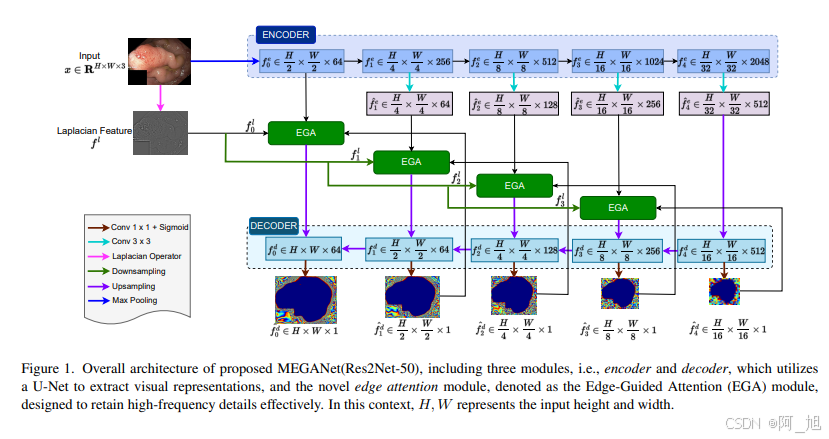
MEGANet是一个端到端的框架,包含三个主要模块:
- 编码器:负责从输入图像中捕获和抽象特征。
- 解码器:专注于提取显著特征,生成与输入图像分辨率匹配的解码图。
- 边缘引导注意力模块(EGA):利用拉普拉斯算子增强边缘信息,确保在解码过程中保留高频细节。
MEGANet通过结合编码器、解码器和EGA模块,能够在多个尺度上保留边缘信息,从而提高了息肉分割的精度。
EGA模块的作用
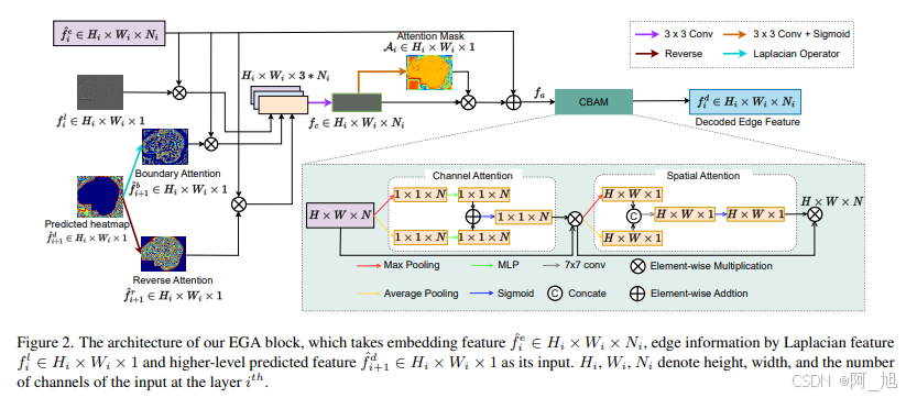
EGA模块的主要作用是通过拉普拉斯算子提取和保留高频边缘信息,增强模型对弱边界的检测能力。具体来说,EGA模块在每一层接收三个输入:
- 编码器特征:来自编码器的视觉特征。
- 高频特征:通过拉普拉斯算子提取的边缘信息。
- 解码器预测特征:来自更高层的解码器预测特征。
EGA模块通过结合这些输入,生成一个融合特征,该特征能够突出边缘细节,并通过注意力机制引导模型关注关键区域,从而提升分割精度。此外,EGA模块还通过卷积块注意力模块(CBAM)进一步校准特征,确保模型能够准确捕捉边界和背景区域的相关性。
总结
MEGANet通过引入EGA模块,有效解决了息肉分割中的弱边界问题,显著提高了分割精度。该方法在多个数据集上的实验结果表明其优越性,为结直肠癌的早期诊断提供了有力的技术支持。
EGA源码与注释
# Github地址:https://github.com/UARK-AICV/MEGANet
# 论文:MEGANet: Multi-Scale Edge-Guided Attention Network for Weak Boundary Polyp Segmentation, WACV 2024
# 论文地址:https://arxiv.org/abs/2309.03329

import torch
import torch.nn.functional as F
import torch.nn as nn

# 定义高斯核函数,用于生成高斯模糊滤波器
def gauss_kernel(channels=3, cuda=True):
    # 创建一个5x5的高斯核
    kernel = torch.tensor([[1., 4., 6., 4., 1],
                           [4., 16., 24., 16., 4.],
                           [6., 24., 36., 24., 6.],
                           [4., 16., 24., 16., 4.],
                           [1., 4., 6., 4., 1.]])
    # 归一化高斯核
    kernel /= 256.
    # 将高斯核扩展到多个通道
    kernel = kernel.repeat(channels, 1, 1, 1)
    if cuda:
        # 如果使用GPU,将高斯核移动到GPU
        kernel = kernel.cuda()
    return kernel

# 定义下采样函数,通过每隔一个像素取值实现
def downsample(x):
    return x[:, :, ::2, ::2]

# 定义卷积高斯模糊函数,使用高斯核对图像进行模糊处理
def conv_gauss(img, kernel):
    # 使用反射填充图像边缘
    img = F.pad(img, (2, 2, 2, 2), mode='reflect')
    # 应用卷积操作进行高斯模糊
    out = F.conv2d(img, kernel, groups=img.shape[1])
    return out

# 定义上采样函数,通过插入零值实现
def upsample(x, channels):
    # 在每个像素之间插入零值
    cc = torch.cat([x, torch.zeros(x.shape[0], x.shape[1], x.shape[2], x.shape[3], device=x.device)], dim=3)
    cc = cc.view(x.shape[0], x.shape[1], x.shape[2] * 2, x.shape[3])
    cc = cc.permute(0, 1, 3, 2)
    cc = torch.cat([cc, torch.zeros(x.shape[0], x.shape[1], x.shape[3], x.shape[2] * 2, device=x.device)], dim=3)
    cc = cc.view(x.shape[0], x.shape[1], x.shape[3] * 2, x.shape[2] * 2)
    x_up = cc.permute(0, 1, 3, 2)
    # 对上采样后的图像应用高斯模糊
    return conv_gauss(x_up, 4 * gauss_kernel(channels))

# 定义拉普拉斯金字塔的一个层级,计算图像与高斯模糊后上采样的图像的差异
def make_laplace(img, channels):
    # 对图像进行高斯模糊
    filtered = conv_gauss(img, gauss_kernel(channels))
    # 对模糊后的图像进行下采样
    down = downsample(filtered)
    # 对下采样后的图像进行上采样
    up = upsample(down, channels)
    # 如果上采样后的图像尺寸与原图不同,进行插值调整
    if up.shape[2] != img.shape[2] or up.shape[3] != img.shape[3]:
        up = nn.functional.interpolate(up, size=(img.shape[2], img.shape[3]))
    # 计算原图与上采样后的图像的差异
    diff = img - up
    return diff

# 构建拉普拉斯金字塔,包含多个层级的差异图像和最终的下采样图像
def make_laplace_pyramid(img, level, channels):
    current = img
    pyr = []
    for _ in range(level):
        # 对当前图像计算拉普拉斯层级
        filtered = conv_gauss(current, gauss_kernel(channels))
        down = downsample(filtered)
        up = upsample(down, channels)
        if up.shape[2] != current.shape[2] or up.shape[3] != current.shape[3]:
            up = nn.functional.interpolate(up, size=(current.shape[2], current.shape[3]))
        diff = current - up
        pyr.append(diff)
        current = down
    # 最后一个层级为最终的下采样图像
    pyr.append(current)
    return pyr

# 定义通道注意力模块,用于计算通道级别的注意力权重
class ChannelGate(nn.Module):
    def __init__(self, gate_channels, reduction_ratio=16):
        super(ChannelGate, self).__init__()
        self.gate_channels = gate_channels
        # 定义MLP网络,用于计算通道注意力权重
        self.mlp = nn.Sequential(
            nn.Flatten(),
            nn.Linear(gate_channels, gate_channels // reduction_ratio),
            nn.ReLU(),
            nn.Linear(gate_channels // reduction_ratio, gate_channels)
        )

    def forward(self, x):
        # 计算平均池化后的通道注意力权重
        avg_out = self.mlp(F.avg_pool2d(x, (x.size(2), x.size(3)), stride=(x.size(2), x.size(3))))
        # 计算最大池化后的通道注意力权重
        max_out = self.mlp(F.max_pool2d(x, (x.size(2), x.size(3)), stride=(x.size(2), x.size(3))))
        # 将平均池化和最大池化后的权重相加
        channel_att_sum = avg_out + max_out

        # 将权重通过sigmoid函数归一化,并扩展到与输入相同的尺寸
        scale = torch.sigmoid(channel_att_sum).unsqueeze(2).unsqueeze(3).expand_as(x)
        # 将权重应用到输入特征图
        return x * scale

# 定义空间注意力模块,用于计算空间级别的注意力权重
class SpatialGate(nn.Module):
    def __init__(self):
        super(SpatialGate, self).__init__()
        kernel_size = 7
        # 定义卷积层,用于计算空间注意力权重
        self.spatial = nn.Conv2d(2, 1, kernel_size, stride=1, padding=(kernel_size - 1) // 2)

    def forward(self, x):
        # 计算最大池化和平均池化后的特征图
        x_compress = torch.cat((torch.max(x, 1)[0].unsqueeze(1), torch.mean(x, 1).unsqueeze(1)), dim=1)
        # 将特征图通过卷积层计算空间注意力权重
        x_out = self.spatial(x_compress)
        # 将权重通过sigmoid函数归一化
        scale = torch.sigmoid(x_out)  # broadcasting
        # 将权重应用到输入特征图
        return x * scale

# 定义CBAM模块,结合通道注意力和空间注意力
class CBAM(nn.Module):
    def __init__(self, gate_channels, reduction_ratio=16):
        super(CBAM, self).__init__()
        # 初始化通道注意力模块
        self.ChannelGate = ChannelGate(gate_channels, reduction_ratio)
        # 初始化空间注意力模块
        self.SpatialGate = SpatialGate()

    def forward(self, x):
        # 应用通道注意力
        x_out = self.ChannelGate(x)
        # 应用空间注意力
        x_out = self.SpatialGate(x_out)
        return x_out

# 定义Edge-Guided Attention Module(EGA)模块,用于结合边缘信息和预测结果进行特征融合
class EGA(nn.Module):
    def __init__(self, in_channels):
        super(EGA, self).__init__()

        # 定义特征融合卷积层
        self.fusion_conv = nn.Sequential(
            nn.Conv2d(in_channels * 3, in_channels, 3, 1, 1),
            nn.BatchNorm2d(in_channels),
            nn.ReLU(inplace=True))

        # 定义注意力机制卷积层
        self.attention = nn.Sequential(
            nn.Conv2d(in_channels, 1, 3, 1, 1),
            nn.BatchNorm2d(1),
            nn.Sigmoid())

        # 初始化CBAM模块
        self.cbam = CBAM(in_channels)

    def forward(self, edge_feature, x, pred):
        residual = x
        xsize = x.size()[2:]

        # 将预测结果通过sigmoid函数归一化
        pred = torch.sigmoid(pred)

        # 计算背景注意力权重
        background_att = 1 - pred
        # 应用背景注意力权重到特征图
        background_x = x * background_att

        # 计算边界注意力权重
        edge_pred = make_laplace(pred, 1)
        # 应用边界注意力权重到特征图
        pred_feature = x * edge_pred

        # 计算高频特征
        edge_input = F.interpolate(edge_feature, size=xsize, mode='bilinear', align_corners=True)
        # 应用高频特征到特征图
        input_feature = x * edge_input

        # 将背景特征、边界特征和高频特征进行拼接
        fusion_feature = torch.cat([background_x, pred_feature, input_feature], dim=1)
        # 应用特征融合卷积层
        fusion_feature = self.fusion_conv(fusion_feature)

        # 计算注意力权重
        attention_map = self.attention(fusion_feature)
        # 应用注意力权重到融合特征
        fusion_feature = fusion_feature * attention_map

        # 将融合特征与残差相加
        out = fusion_feature + residual
        # 应用CBAM模块
        out = self.cbam(out)
        return out

if __name__ == '__main__':
    # 模拟输入张量
    edge_feature = torch.randn(1, 1, 128, 128).cuda()
    x = torch.randn(1, 64, 128, 128).cuda()
    pred = torch.randn(1, 1, 128, 128).cuda()  # pred 通常是1通道

    # 实例化 EGA 类
    block = EGA(64).cuda()

    # 传递输入张量通过 EGA 实例
    output = block(edge_feature, x, pred)

    # 打印输入和输出的形状
    print(edge_feature.size())
    print(x.size())
    print(pred.size())
    print(output.size())
好了,这篇文章就介绍到这里,喜欢的小伙伴感谢给点个赞和关注,更多精彩内容持续更新~~
关于本篇文章大家有任何建议或意见,欢迎在评论区留言交流!