http://www0.cs.ucl.ac.uk/staff/d.silver/web/Teaching.html
引自Reinforcement Learning:An Introduction强化学习名著2018新编版
DPG论文http://www0.cs.ucl.ac.uk/staff/d.silver/web/Applications_files/deterministic-policy-gradients.pdf
PolicyGradient论文https://www.ics.uci.edu/~dechter/courses/ics-295/winter-2018/papers/2000-nips12-sutton-mcallester-policy-gradient-methods-for-reinforcement-learning-with-function-approximation.pdf
DDPG论文http://www0.cs.ucl.ac.uk/staff/d.silver/web/Applications_files/ddpg.pdf
DQN论文http://web.cse.ohio-state.edu/~wang.7642/homepage/files/Peidong_Wang_DQN.pdf

【强化学习】DDPG(Deep Deterministic Policy Gradient)算法详解

之前我们在Actor-Critic上面提到过了DDPG，现在本篇详细讲解，因为Actor-Critic收敛慢的问题所以Deepmind 提出了 Actor Critic 升级版 Deep Deterministic Policy Gradient，后者融合了 DQN 的优势, 解决了收敛难的问题。

1、算法思想

DDPG我们可以拆开来看Deep Deterministic Policy Gradient
这里写图片描述
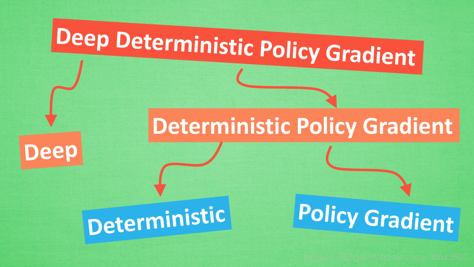
Deep：首先Deep我们都知道，就是更深层次的网络结构，我们之前在DQN中使用两个网络与经验池的结构，在DDPG中就应用了这种思想。
PolicyGradient：顾名思义就是策略梯度算法，能够在连续的动作空间根据所学习到的策略（动作分布）随机筛选动作
Deterministic : 它的作用就是用来帮助Policy Gradient不让他随机选择，只输出一个动作值

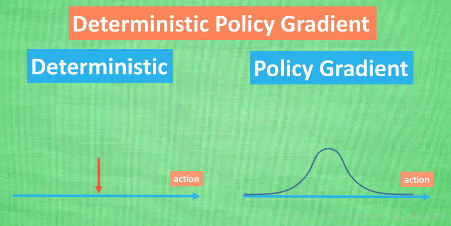
随机性策略， $\sum\pi(a|s)=1$ 策略输出的是动作的概率，使用正态分布对动作进行采样选择，即每个动作都有概率被选到；优点，将探索和改进集成到一个策略中；缺点，需要大量训练数据。
确定性策略， $\pi(s) S→A$ 策略输出即是动作；优点，需要采样的数据少，算法效率高；缺点，无法探索环境。然而因为我们引用了DQN的结构利用offPolicy采样，这样就解决了无法探索环境的问题

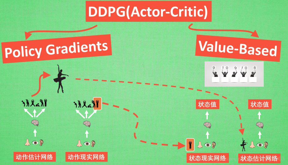
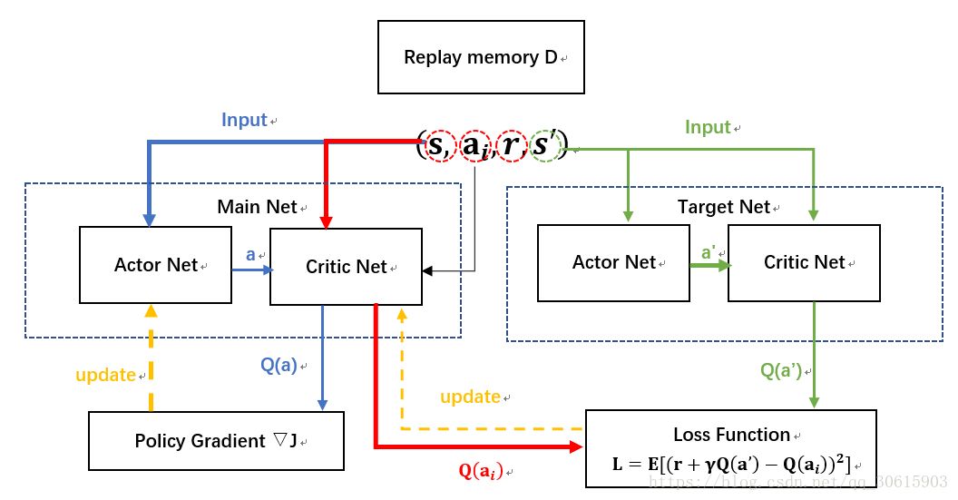
从DDPG网络整体上来说：他应用了 Actor-Critic 形式的, 所以也具备策略 Policy 的神经网络和基于价值 Value 的神经网络，因为引入了DQN的思想，每种神经网络我们都需要再细分为两个, Policy Gradient 这边，我们有估计网络和现实网络，估计网络用来输出实时的动作, 供 actor 在现实中实行，而现实网络则是用来更新价值网络系统的。再看另一侧价值网络, 我们也有现实网络和估计网络, 他们都在输出这个状态的价值, 而输入端却有不同, 状态现实网络这边会拿着从动作现实网络来的动作加上状态的观测值加以分析，而状态估计网络则是拿着当时 Actor 施加的动作当做输入。

DDPG 在连续动作空间的任务中效果优于DQN而且收敛速度更快，但是不适用于随机环境问题。

2、公式推导

再来啰唆一下前置公式
$s_t$ ：在t时刻，agent所能表示的环境状态，比如观察到的环境图像，agent在环境中的位置、速度、机器人关节角度等；
$a_t$ ：在t时刻，agent选择的行为（action）
$r(s_t,a_t)$ ：函数: 环境在状态st 执行行为at后，返回的单步奖励值；
$R_t$ ：是从当前状态直到将来某个状态中间所有行为所获得奖励值的之和当然下一个状态的奖励值要有一个衰变系数 $\gamma$ 一般情况下可取0到1的小数
$R_t=∑_{i=t}γ^{i−t}r(s_i,a_i)$

Policy Gradient：
通过概率的分布函数确定最优策略，在每一步根据该概率分布获取当前状态最佳的动作，产生动作采取的是随机性策略
$a_t ∼π_θ(s_t|θ^π)$
目标函数： $J(\pi_\theta)=∫_Sρ^\pi(s)∫_A\pi_\theta(s,a)r(s,a)dads=E_{s∼ρ^\pi,a∼\pi_\theta}[r(s,a)]$ （注意dads不是什么未知的符号，而是积分的 da ds）
梯度： $∇_θJ(π_θ)=∫_Sρ^\pi(s)∫_A∇_θ\pi_\theta(s,a)Q^\pi(s,a)dads=E_{s∼ρ^\pi,a∼\pi_\theta}[∇_θlog\pi_\theta(a|s)Q^\pi(s,a)]$

Deterministic Policy Gradient：
因为Policy Gradient是采取随机性策略，所以要想获取当前动作action就需要对最优策略的概率分布进行采样，而且在迭代过程中每一步都要对整个动作空间进行积分，所以计算量很大
在PG的基础上采取了确定性策略，根据行为直接通过函数μ确定了一个动作，可以吧μ理解成一个最优行为策略

$a_t=μ(s_t|θ^μ)$

performance objective为
$J(μ_\theta)=∫_Sρ^μ(s)r(s,μ_\theta(s))ds$
$J(μ_\theta)=E_{s∼ρ^μ}[r(s,μ_\theta(s))]$
deterministic policy梯度
$▽_\theta J(μ_\theta)=∫_Sρ^μ(s)▽\theta μ_\theta(s)Q^μ(s,a)|_{a=μ_\theta}ds=E_{s∼ρ^β}[▽\theta μ_\theta(s)Q^μ(s,a)|_{a=μ_\theta}]$

DDPG就是用了确定性策略在DPG基础上结合DQN的特点建议改进出来的算法

Deep Deterministic Policy Gradient
所以基于上述两种算法
DDPG采用确定性策略μ来选取动作 $a_t=μ(s_t|θ^μ)$ 其中 $θ^μ$ 是产生确定性动作的策略网络的参数。根据之前提到过的AC算与PG算法我们可以想到，使用策略网络μ来充当actor，使用价值网络来拟合(s,a)函数，来充当critic的角色，所以将DDPG的目标函数就可以定义为

$J(θ^μ)=E_{θ^μ}[r_1+γr_2+γ^2r_3+⋯]$

此时Q函数表示为在采用确定性策略μ下选择动作的奖励期望值，在DDPG我们就采用DQN的结构使用Q网络来拟合Q函数

$Q^μ(s_t,a_t)=E [r(s_t,a_t)+γQ^μ(s_{t+1},μ(s_{t+1}))]$

Q网络中的参数定义为 $\theta^Q$ ， $Q^μ(s,μ(s))$ 表示使用μ策略在s状态选选取动作所获取的回报期望值，又因为是在连续空间内所以期望可用积分来求，则可以使用下式来表示策略μ的好坏

$J_β(μ)=∫_Sρ^β(s)Q^μ(s,μ(s))ds=E_{s∼ρ^β}[Q^μ(s,μ(s)]$

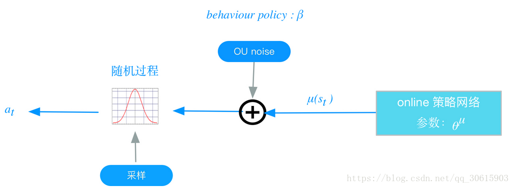
behavior policy β: 在常见的RL训练过程中存在贪婪策略来平衡exploration和exploit与之类似，在DDPG中使用Uhlenbeck-Ornstein随机过程（下面简称UO过程），作为引入的随机噪声：UO过程在时序上具备很好的相关性，可以使agent很好的探索具备动量属性的环境exploration的目的是探索潜在的更优策略，所以训练过程中，我们为action的决策机制引入随机噪声：
过程如下图所示：
这里写图片描述

Silver大神证明了目标函数采用μ策略的梯度与Q函数采用μ策略的期望梯度是等价的：

$\frac{∂J(θ^μ)}{∂θ^μ}=E_s[\frac{∂Q(s,a|θ^Q)}{∂θ^μ}]$

因为是确定性策略 $a=μ(s|θ^μ)$ 所以得到Actor网络的梯度为

$\frac{∂J(θ^μ)}{∂θ^μ}=E_s[\frac{∂Q(s,a|θ^Q)}{∂a} \frac{∂π(s|θ^μ)}{∂θ^μ}]$

$▽_\theta J_β(μ_\theta)=∫_Sρ^β(s)▽_\theta μ_\theta(s)Q^μ(s,a)|_{a=μ_\theta}ds=E_{s∼ρ^β}[▽_\theta μ_\theta(s)Q^μ(s,a)|_{a=μ_\theta}]$

在另一方面Critic网络上的价值梯度为
$\frac{∂L(θ^Q)}{∂θ^Q}=E_{s,a,r,s′∼D}[(TargetQ−Q(s,a|θ^Q)\frac{∂Q(s,a|θ^Q)}{∂θ^Q}]$
$TargetQ=r+γQ′(s′,π(s′|θ^{μ′})|θ^{Q′})$

损失函数采取均方误差损失MSE，另外在计算策略梯度期望的时候仍然选择蒙特卡罗法来取无偏估计（随机采样加和平均法）

我们有了上述两个梯度公式就可以使用梯度下降进行网络的更新
网络结构图如下因为引用了DQN的结构，所以就多了一个target网络
这里写图片描述

3、代码实现

https://morvanzhou.github.io/tutorials/引用morvan老师的源码

import tensorflow as tf
import numpy as np
import gym
import time


#####################  hyper parameters  ####################

MAX_EPISODES = 200
MAX_EP_STEPS = 200
LR_A = 0.001    # learning rate for actor
LR_C = 0.002    # learning rate for critic
GAMMA = 0.9     # reward discount
TAU = 0.01      # soft replacement
MEMORY_CAPACITY = 10000
BATCH_SIZE = 32

RENDER = False
ENV_NAME = 'Pendulum-v0'


###############################  DDPG  ####################################


class DDPG(object):
    def __init__(self, a_dim, s_dim, a_bound,):
        self.memory = np.zeros((MEMORY_CAPACITY, s_dim * 2 + a_dim + 1), dtype=np.float32)
        self.pointer = 0
        self.sess = tf.Session()

        self.a_dim, self.s_dim, self.a_bound = a_dim, s_dim, a_bound,
        self.S = tf.placeholder(tf.float32, [None, s_dim], 's')
        self.S_ = tf.placeholder(tf.float32, [None, s_dim], 's_')
        self.R = tf.placeholder(tf.float32, [None, 1], 'r')

        self.a = self._build_a(self.S,)
        q = self._build_c(self.S, self.a, )
        a_params = tf.get_collection(tf.GraphKeys.TRAINABLE_VARIABLES, scope='Actor')
        c_params = tf.get_collection(tf.GraphKeys.TRAINABLE_VARIABLES, scope='Critic')
        ema = tf.train.ExponentialMovingAverage(decay=1 - TAU)          # soft replacement

        def ema_getter(getter, name, *args, **kwargs):
            return ema.average(getter(name, *args, **kwargs))

        target_update = [ema.apply(a_params), ema.apply(c_params)]      # soft update operation
        a_ = self._build_a(self.S_, reuse=True, custom_getter=ema_getter)   # replaced target parameters
        q_ = self._build_c(self.S_, a_, reuse=True, custom_getter=ema_getter)

        a_loss = - tf.reduce_mean(q)  # maximize the q
        self.atrain = tf.train.AdamOptimizer(LR_A).minimize(a_loss, var_list=a_params)

        with tf.control_dependencies(target_update):    # soft replacement happened at here
            q_target = self.R + GAMMA * q_
            td_error = tf.losses.mean_squared_error(labels=q_target, predictions=q)
            self.ctrain = tf.train.AdamOptimizer(LR_C).minimize(td_error, var_list=c_params)

        self.sess.run(tf.global_variables_initializer())

    def choose_action(self, s):
        return self.sess.run(self.a, {self.S: s[np.newaxis, :]})[0]

    def learn(self):
        indices = np.random.choice(MEMORY_CAPACITY, size=BATCH_SIZE)
        bt = self.memory[indices, :]
        bs = bt[:, :self.s_dim]
        ba = bt[:, self.s_dim: self.s_dim + self.a_dim]
        br = bt[:, -self.s_dim - 1: -self.s_dim]
        bs_ = bt[:, -self.s_dim:]

        self.sess.run(self.atrain, {self.S: bs})
        self.sess.run(self.ctrain, {self.S: bs, self.a: ba, self.R: br, self.S_: bs_})

    def store_transition(self, s, a, r, s_):
        transition = np.hstack((s, a, [r], s_))
        index = self.pointer % MEMORY_CAPACITY  # replace the old memory with new memory
        self.memory[index, :] = transition
        self.pointer += 1

    def _build_a(self, s, reuse=None, custom_getter=None):
        trainable = True if reuse is None else False
        with tf.variable_scope('Actor', reuse=reuse, custom_getter=custom_getter):
            net = tf.layers.dense(s, 30, activation=tf.nn.relu, name='l1', trainable=trainable)
            a = tf.layers.dense(net, self.a_dim, activation=tf.nn.tanh, name='a', trainable=trainable)
            return tf.multiply(a, self.a_bound, name='scaled_a')

    def _build_c(self, s, a, reuse=None, custom_getter=None):
        trainable = True if reuse is None else False
        with tf.variable_scope('Critic', reuse=reuse, custom_getter=custom_getter):
            n_l1 = 30
            w1_s = tf.get_variable('w1_s', [self.s_dim, n_l1], trainable=trainable)
            w1_a = tf.get_variable('w1_a', [self.a_dim, n_l1], trainable=trainable)
            b1 = tf.get_variable('b1', [1, n_l1], trainable=trainable)
            net = tf.nn.relu(tf.matmul(s, w1_s) + tf.matmul(a, w1_a) + b1)
            return tf.layers.dense(net, 1, trainable=trainable)  # Q(s,a)


###############################  training  ####################################

env = gym.make(ENV_NAME)
env = env.unwrapped
env.seed(1)

s_dim = env.observation_space.shape[0]
a_dim = env.action_space.shape[0]
a_bound = env.action_space.high

ddpg = DDPG(a_dim, s_dim, a_bound)

var = 3  # control exploration
t1 = time.time()
for i in range(MAX_EPISODES):
    s = env.reset()
    ep_reward = 0
    for j in range(MAX_EP_STEPS):
        if RENDER:
            env.render()

        # Add exploration noise
        a = ddpg.choose_action(s)
        a = np.clip(np.random.normal(a, var), -2, 2)    # add randomness to action selection for exploration
        s_, r, done, info = env.step(a)

        ddpg.store_transition(s, a, r / 10, s_)

        if ddpg.pointer > MEMORY_CAPACITY:
            var *= .9995    # decay the action randomness
            ddpg.learn()

        s = s_
        ep_reward += r
        if j == MAX_EP_STEPS-1:
            print('Episode:', i, ' Reward: %i' % int(ep_reward), 'Explore: %.2f' % var, )
            # if ep_reward > -300:RENDER = True
            break

print('Running time: ', time.time() - t1)