Logistic Regression逻辑回归---梯度下降求解

Logistic Regression逻辑回归—梯度下降求解

里面一些公式的推导，我有空了就会再写一篇博客
机器学习入门，这个比较简单，易懂。
链接：https://pan.baidu.com/s/1nwKe0g-U7KRoGVoTwz_fWw 密码：9ucp

问题描述

建立一个逻辑回归模型来预测一个学生是否被大学录取。
根据两次考试的结果来决定申请人是否被录取
我们拥有以前学生的历史数据，将它作为逻辑回归的训练集。（看图三）
对于每一个培训例子，决定出是否能被录取。
let’s 建立一个分类模型，根据你的考试成绩估计你能不能被录取。录取—1，未录取—0

1.数据长什么样子呢？？？

（1）用pandas读出数据

我们要用的数据，可以观察到 没有列名，这是个什么鬼，仔细观察仔细仔细仔细

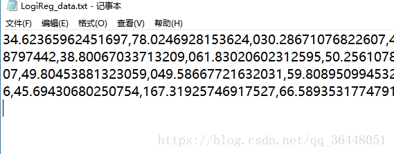
34.62365962451697,78.0246928153624,0
30.28671076822607,43.89499752400101,0
… 发现没有，仔细看
我们要用的数据，可以观察到 有三列，没有列名 ，要自己指定

import numpy as np
import pandas as pd
import matplotlib.pyplot as plt
import os
#path = 'data' + os.sep + 'LogiReg_data.txt' #os.sep路径分隔符
path = 'LogiReg_data.txt'
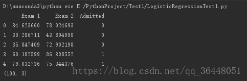
pdData = pd.read_csv(path, header=None, names=['Exam 1', 'Exam 2', 'Admitted'])
print(pdData.head()) #打印前5条样本
print(pdData.shape) #打印出数据维度 100行3列

有100个样本 每个样本有三个数据

（2）用matplotlib作图刻画数据（散点图scatter）

s–指描点的大小，
c–指颜色， 正例（录取）用蓝色 —————-反例（未录取）用红色
marker–指样式，正例（录取）用o圈圈 —— 反例（未录取）用x 叉叉

positive = pdData[pdData['Admitted'] == 1]
# 正例returns the subset of rows such Admitted = 1, i.e. the set of *positive* examples
negative = pdData[pdData['Admitted'] == 0]
# 反例returns the subset of rows such Admitted = 0, i.e. the set of *negative* examples

fig, ax = plt.subplots(figsize=(10, 5)) #figsize指定画图域
ax.scatter(positive['Exam 1'], positive['Exam 2'], s=30, c='b', marker='o', label='Admitted')
ax.scatter(negative['Exam 1'], negative['Exam 2'], s=30, c='r', marker='x', label='Not Admitted')
ax.legend()
ax.set_xlabel('Exam 1 Score')
ax.set_ylabel('Exam 2 Score')
plt.show()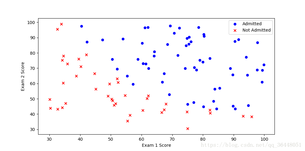

我们可以粗略的观察到录取与未录取之间有个分界线，接下来要做的就是求解两门考试成绩与录取之间的关系函数

2.The logistic regression

我们这样想：

$$(录取/不录取)=\theta_0+\theta_1x_1+\theta_2x_2$$

现在就是根据已有的数据怼出一个函数来，把你的两门成绩往这函数里一套，就知道你能不能被录取了。

目标：建立分类器（求解出三个参数$θ_0 θ_1 θ_2$ ）
设定阈值，根据阈值判断录取结果 ： 大于0.5 认为被录取； 否则未被录取

要完成的模块

sigmoid : 映射到概率的函数 预测结果值到概率的转换
model : 返回预测结果值
cost : 根据参数计算损失
gradient : 计算每个参数的梯度方向
descent : 进行参数更新
accuracy: 计算精度

2.1 sigmoid 函数

这个公式是历史的总结。我们只要知道它可以把预测值转换为概率值。你看它的性质就知道了。你随便输个数，它都能给你转成[0 ,1]的数。（看下面的图）

那为什么要转成概率值？有了概率值，你就可以划界线概率值>=0.5，我就认为结果是1（录取），否则我就认为结果是0.——– 二分类

$$g(z)=\frac{1}{1+e^{−z}}$$

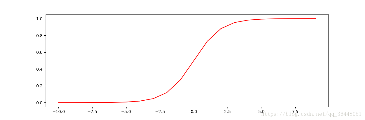
性质：
$值域[0, 1]$
$g(0)=0.5$
$g(-\infty)=0$
$g(+\infty)=1$

def sigmoid(z):
    return 1 / (1 + np.exp(-z))

2.2 model函数

model函数就是$h_\theta(x)$
在建立回归模型的时候，要在数据中插入一列，那一列值都等于1。把数值运算转为矩阵运算

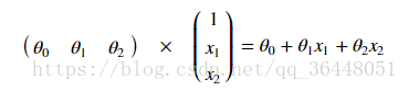
#X是数据，theta是参数，np.dot矩阵乘法
def model(X, theta):
    return sigmoid(np.dot(X, theta.T))


pdData.insert(0, 'Ones', 1) # in a try / except structure so as not to return an error if the block si executed several times
#新加一列 命名为Ones 填充值为1
# set X (training data) and y (target variable)
orig_data = pdData.as_matrix()
cols = orig_data.shape[1]
X = orig_data[:, 0:cols-1]  #数据
y = orig_data[:, cols-1:cols] #真实值 0或者1 没录取/录取
theta = np.zeros([1, 3])  #占位 创建一行三列的theta参数 ，填充为0

我们打印X，y，theta看一下

2.3 cost损失函数

对数似然函数

$$l(\theta)=logL(\theta)=\sum_{i=0}^m\Bigl(ylog\bigl(h_\theta(x_i)\bigr)+(1-y)log\bigl(1-h_\theta(x_i)\bigr)\Bigr)$$
求平均损失
$$J(\theta)=-\frac{1}{m}l(\theta)$$

def cost(X, y, theta):
    left = np.multiply(y, np.log(model(X, theta)))
    right = np.multiply(1 - y, np.log(1 - model(X, theta)))
    return -np.sum(left + right) / (len(X))
#print(cost(X, y, theta))

$h_\theta(x_i)$调用model函数求

2.4 gradient 函数计算梯度

有3个$\theta$参数，所以就求出3个梯度出来。$\theta_j$就表示第j个参数
对$J(\theta)$求偏导

$$\frac{\partial J(\theta) }{\partial\theta_j}=\frac{1}{m}\sum_{i=0}^m\Bigl(\bigl(h_\theta(x_i)\bigr)-y_i\Bigr)x_i^j$$
$x_i^j$是指第i个样本第 j 列

def gradient(X, y, theta):
    grad = np.zeros(theta.shape)  #一行三列
    error = (model(X, theta) - y).ravel()  # ravel 将多维数组降为一维
    for j in range(len(theta.ravel())):  # for each parmeter
        term = np.multiply(error, X[:, j])  # X[:, j]取第j列的所有样本
        grad[0, j] = np.sum(term) / len(X)

    return grad

2.5 descent函数进行参数的更新 梯度下降

2.5.1 打乱数据

#洗牌 打乱数据顺序，使模型泛化能力更强
def shuffleData(data):
    np.random.shuffle(data)
    cols = data.shape[1]
    X = data[:, 0:cols-1]
    y = data[:, cols-1:]
    return X, y

2.5.2 梯度下降和停止策略
不可能让函数不停的执行下去，所以要设置停止策略

三种梯度下降方法：

• 批量梯度下降
• 随机梯度下降
• 小批量梯度下降

三种停止策略

• 设定迭代次数
• 根据损失值停止
• 根据梯度变化停止

STOP_ITER = 0  #设定确定的迭代次数
STOP_COST = 1  #根据损失值停止。迭代的目标函数之间差异特别小特别小，就可以停止了
STOP_GRAD = 2  #根据梯度变化停止，两次算的梯度没啥变化了，可停止

def stopCriterion(type, value, threshold):
    #设定三种不同的停止策略
    if type == STOP_ITER:
        return value > threshold
    elif type == STOP_COST:
        return abs(value[-1]-value[-2]) < threshold
    elif type == STOP_GRAD:
        return np.linalg.norm(value) < threshold

2.5.3 梯度下降求解
参数更新：

$$\theta_j:=\theta_j-\alpha\frac{1}{m}\sum_{i=1}^{m}\Bigl(h_\theta(x_i)-y_i\Bigr)x_i^j$$
其中： $\frac{1}{m}\sum_{i=1}^{m}\Bigl(h_\theta(x_i)-y_i\Bigr)x_i^j$是函数gradient(X, y, theta)的返回值grad，也就是更新方向
$\alpha$是学习率，也就是更新力度
减号-代表梯度下降

def descent(data, theta, batchSize, stopType, thresh, alpha):
    # 梯度下降求解
    init_time = time.time()
    i = 0  # 迭代次数
    k = 0  # batch
    X, y = shuffleData(data)
    grad = np.zeros(theta.shape)  # 计算的梯度
    costs = [cost(X, y, theta)]  # 损失值

    while True: #数次迭代
        grad = gradient(X[k:k + batchSize], y[k:k + batchSize], theta)
        k += batchSize  # 取batch数量个数据
        if k >= m:
            k = 0
            X, y = shuffleData(data)  # 重新洗牌
        theta = theta - alpha * grad  # 参数更新
        costs.append(cost(X, y, theta))  # 计算新的损失
        i += 1
#停止策略，什么时候该停止
        if stopType == STOP_ITER:
            value = i
        elif stopType == STOP_COST:
            value = costs
        elif stopType == STOP_GRAD:
            value = grad
        if stopCriterion(stopType, value, thresh):
            break

    return theta, i - 1, costs, grad, time.time() - init_time

2.5.4 画图的功能性函数

#画图的功能性函数
def runExpe(data, theta, batchSize, stopType, thresh, alpha):
    #import pdb; pdb.set_trace();
    theta, iter, costs, grad, dur = descent(data, theta, batchSize, stopType, thresh, alpha)
    name = "Original" if (data[:, 1] > 2).sum() > 1 else "Scaled"
    name += " data - learning rate: {} - ".format(alpha)
    if batchSize == m:
        strDescType = "Gradient"
    elif batchSize == 1: #随机梯度下降
        strDescType = "Stochastic"
    else:                #小批量梯度下降
        strDescType = "Mini-batch ({})".format(batchSize)

    name += strDescType + " descent - Stop: "
    if stopType == STOP_ITER:
        strStop = "{} iterations".format(thresh)
    elif stopType == STOP_COST:
        strStop = "costs change < {}".format(thresh)
    else:
        strStop = "gradient norm < {}".format(thresh)
    name += strStop

    print("***{}\nTheta: {} - Iter: {} - Last cost: {:03.2f} - Duration: {:03.2f}s".format(
        name, theta, iter, costs[-1], dur))
    fig, ax = plt.subplots(figsize=(12, 4))
    ax.plot(np.arange(len(costs)), costs, 'r')
    ax.set_xlabel('Iterations')
    ax.set_ylabel('Cost')
    ax.set_title(name.upper() + ' - Error vs. Iteration')
    plt.show()
    return theta

3 Try一Try对比一下

3.1 batchSize=m,批量梯度下降

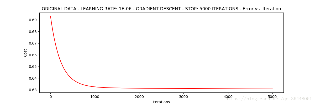
3.1.1 停止策略：STOP_ITER设定迭代次数
thresh迭代5000次
学习率为0.000001

m=100#共有100个样本数据
print(runExpe(orig_data, theta, m, STOP_ITER, thresh=5000, alpha=0.000001))`这里写代码片`

结果如下：
***Original data - learning rate: 1e-06 - Gradient descent - Stop: 5000 iterations
Theta: [[-0.00027127 0.00705232 0.00376711]] - Iter: 5000 - Last cost: 0.63 - Duration: 1.01s
[[-0.00027127 0.00705232 0.00376711]]

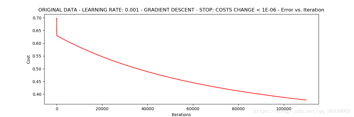
3.1.2 停止策略：STOP_COST 根据损失值停止
thresh 设定阈值1E-6 学习率：0.001

m=100
print(runExpe(orig_data, theta, m, STOP_COST, thresh=0.000001, alpha=0.001))

结果如下：
***Original data - learning rate: 0.001 - Gradient descent - Stop: costs change < 1e-06
Theta: [[-5.13364014 0.04771429 0.04072397]] - Iter: 109901 - Last cost: 0.38 - Duration: 25.64s
[[-5.13364014 0.04771429 0.04072397]]

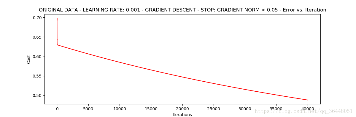
3.1.3 停止策略：STOP_GRAD 根据梯度停止
thresh 设定阈值0.05 学习率0.001

m=100
print(runExpe(orig_data, theta, m, STOP_GRAD, thresh=0.05, alpha=0.001))

结果如下：
***Original data - learning rate: 0.001 - Gradient descent - Stop: gradient norm < 0.05
Theta: [[-2.37033409 0.02721692 0.01899456]] - Iter: 40045 - Last cost: 0.49 - Duration: 8.42s
[[-2.37033409 0.02721692 0.01899456]]

3.2 Stochastic descent 随机梯度下降

3.2.1 停止策略：STOP_ITER 设定迭代次数
10000次迭代 学习率0.001

print(runExpe(orig_data, theta, 1, STOP_ITER, thresh=10000, alpha=0.001))

结果如下：
***Original data - learning rate: 0.001 - Stochastic descent - Stop: 10000 iterations
Theta: [[-0.75604928 0.07985166 -0.08463065]] - Iter: 10000 - Last cost: 1.31 - Duration: 0.62s
[[-0.75604928 0.07985166 -0.08463065]]

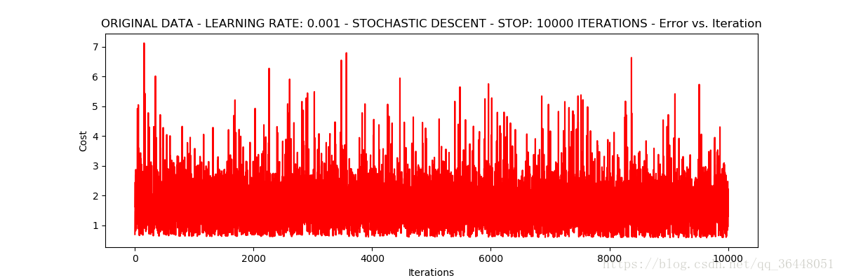
发现很不稳定，我们再把学习率调小，迭代次数增多

print(runExpe(orig_data, theta, 1, STOP_ITER, thresh=15000, alpha=0.000001))

结果：
***Original data - learning rate: 1e-06 - Stochastic descent - Stop: 15000 iterations
Theta: [[-0.00097123 0.00894949 0.00196817]] - Iter: 15000 - Last cost: 0.63 - Duration: 0.97s
[[-0.00097123 0.00894949 0.00196817]]

任然不是很好

3.3 Mini-batch descent 小批量梯度下降

batchSize=64 迭代15000次，学习率0.001

print(runExpe(orig_data, theta, 64, STOP_ITER, thresh=15000, alpha=0.001))

结果如下：
***Original data - learning rate: 0.001 - Mini-batch (64) descent - Stop: 15000 iterations
Theta: [[-1.00810559 0.02079828 0.00950968]] - Iter: 15000 - Last cost: 0.57 - Duration: 2.03s
[[-1.00810559 0.02079828 0.00950968]]

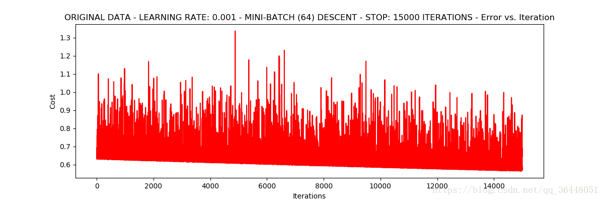
还是不稳

浮动仍然比较大，我们来尝试对数据进行标准化。 将数据按其属性(按列进行)减去其均值，然后除以其方差。最后得到的结果是，对每个属性/每列来说所有数据都聚集在0附近，方差值为1

3.4数据标准化的try

（1）

from sklearn import preprocessing as pp
scaled_data = orig_data.copy()
scaled_data[:, 1:3] = pp.scale(orig_data[:, 1:3])
print(runExpe(scaled_data, theta, m, STOP_ITER, thresh=5000, alpha=0.001))

结果如下：
***Scaled data - learning rate: 0.001 - Gradient descent - Stop: 5000 iterations
Theta: [[0.3080807 0.86494967 0.77367651]] - Iter: 5000 - Last cost: 0.38 - Duration: 0.98s
[[0.3080807 0.86494967 0.77367651]]

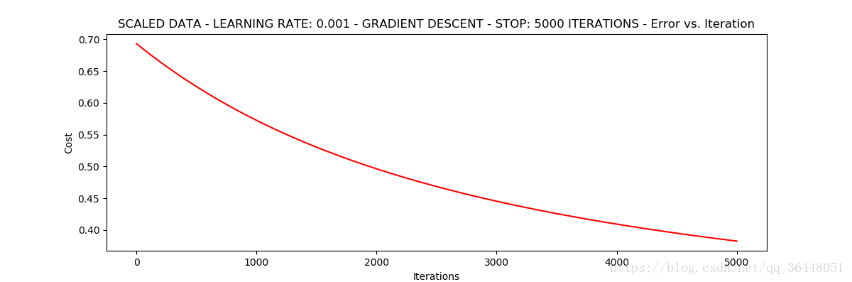
可以看到 ，经过标准化后 只迭代了5000次，学习率为0.001 ，就的得到了比较好的结果。Last cost 为0.38，比之前的结果都小。

数据预处理很重要
（2）批量梯度下降

print(runExpe(scaled_data, theta, m, STOP_GRAD, thresh=0.02, alpha=0.001))

结果如下：
***Scaled data - learning rate: 0.001 - Gradient descent - Stop: gradient norm < 0.02
Theta: [[1.0707921 2.63030842 2.41079787]] - Iter: 59422 - Last cost: 0.22 - Duration: 13.64s
[[1.0707921 2.63030842 2.41079787]]

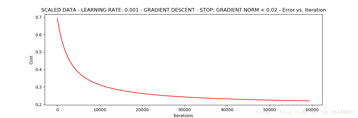
这次更小了，到了0.22。 总共迭代了59422次。那我们继续

（3）

print(runExpe(scaled_data, theta, 1, STOP_GRAD, thresh=0.002/5, alpha=0.001))

结果如下：

***Scaled data - learning rate: 0.001 - Stochastic descent - Stop: gradient norm < 0.0004
Theta: [[1.14927712 2.7915126 2.56576219]] - Iter: 72545 - Last cost: 0.22 - Duration: 5.39s
对比（2）；同样达到cost 0.22的效果（3）的时间消耗更短，但迭代次数也变得很多。接下来我们看看mini-batch
（4）Mini-batch，C位出道

print(runExpe(scaled_data, theta, 16, STOP_GRAD, thresh=0.002, alpha=0.1))

结果如下：

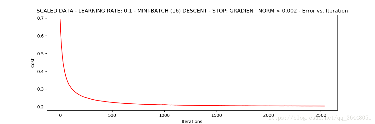
***Scaled data - learning rate: 0.1 - Mini-batch (16) descent - Stop: gradient norm < 0.002
Theta: [[1.54395782 3.69046789 3.44571026]] - Iter: 2533 - Last cost: 0.20 - Duration: 0.26s

mini-batch很不错，1154次迭代，达到0.20，不过每次执行结果会有一些不同，迭代次数有700多的，有2000多的；cost要么0.20，要么0.21；在最终精确度上有时89%有时90%

3.5 精确度

逻辑回归得到的是概率值 怎么把它变成类别值
设定阈值：>=0.5 返回1 ，录取
<0.5 返回0 ，不录取

    #设定阈值
def predict(X, theta):
    return [1 if x >= 0.5 else 0 for x in model(X, theta)]

theta = runExpe(scaled_data, theta, 16, STOP_GRAD, thresh=0.002, alpha=0.1)
scaled_X = scaled_data[:, :3]
y = scaled_data[:, 3]
predictions = predict(scaled_X, theta)
correct = [1 if ((a == 1 and b == 1) or (a == 0 and b == 0)) else 0 for (a, b) in zip(predictions, y)]
accuracy = (sum(map(int, correct)) % len(correct))
print('accuracy = {0}%'.format(accuracy))

accuracy = 90%
三个参数值：
theta=[[1.4609743 3.44657722 3.24588964]]
在100个样本中，正确预测的概率是90%左右

总结一下

1. 了解数据
2. 数据预处理
3. 三种梯度下降方法三种迭代停止策略，多试几次选择最佳的方案，mini-batch是首选。学习率alpha和阈值thresh的大小多试几次。用Mini-batch时的batchSize一般情况下选16，32，64，128。常用64。越大的batch结果越稳定
4. 反正就是try一try
5. 希望对你的学习有所帮助

代码可以到这里下载，这里写链接内容 或者留下你的联系方式，我发给你。

完成！！！