灵感:利用CNN网络从医学图像中检测和分类人类疾病的自动化方法。
1、首先我们先对图片进行相应的分析,胸部X线影像(前 - 后)选自广州市广州妇女儿童医学中心一至五岁儿科患者的胸透图片。总共有5840张图片,用其中的5216张用于训练模型,614用于测试,训练集中有3875张是患有肺炎的图片,1341张是正常的。所有胸部X射线成像均作为患者常规临床护理的一部分判定之一。
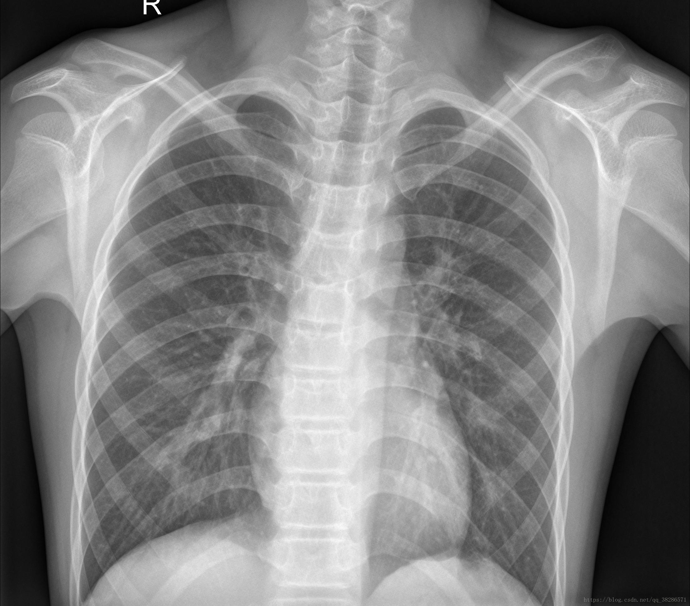
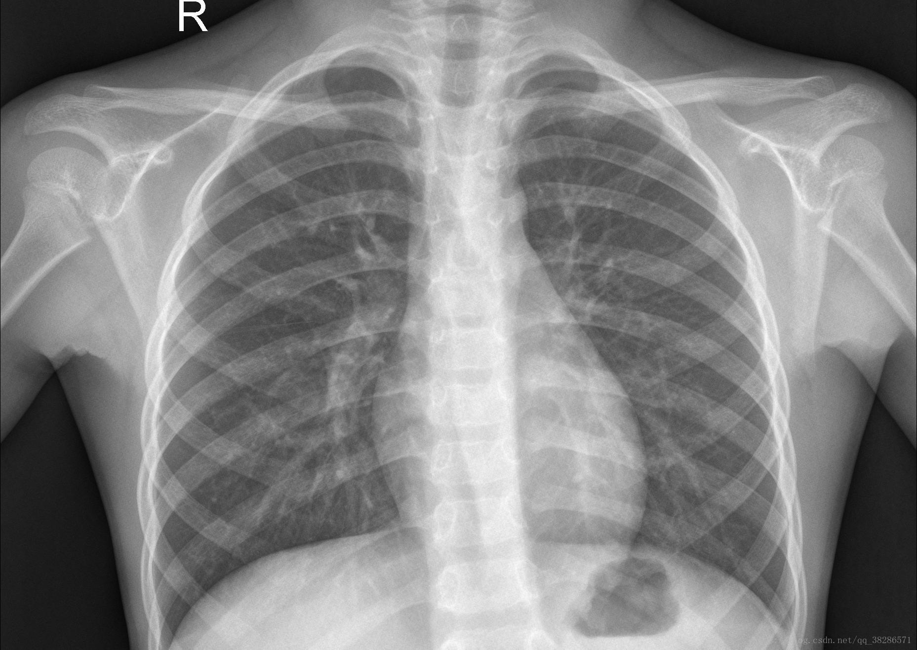
如下图为随机的两张正常的X射线图片
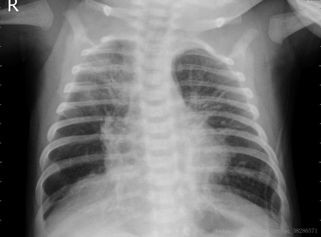
下面的是患有肺炎的X射线图
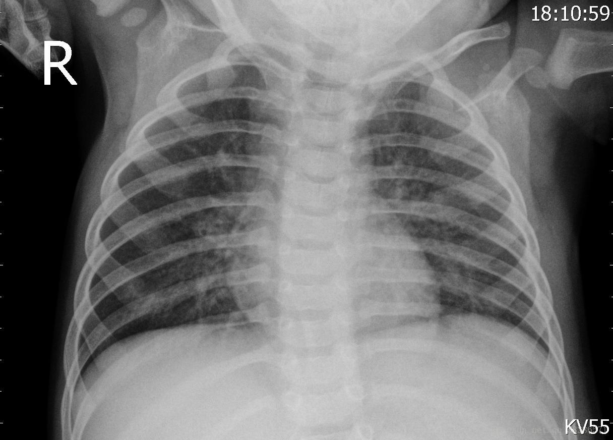
对于非专业的人来说,完全无法分辨是否患有肺炎。如果使用机器学习中的CNN网络实现对肺炎图片的分类,将会在很大程度上减少医生的工作量。
本次数据集分为3个文件夹(train,test,val(本次程序验证集直接使用的测试集)),并包含每个图像类别(Pneumonia / Normal)的子文件夹。有5,863个X射线图像(JPEG)和2个类别(肺炎/正常)。
相应的代码实现如下:
import numpy as np
from tensorflow.python import keras
from keras import layers
from keras.models import Model, Sequential
from keras.optimizers import Adam
from keras.preprocessing.image import ImageDataGenerator
from sklearn.metrics import classification_report, confusion_matrix
from mlxtend.plotting import plot_confusion_matrix
import matplotlib.pyplot as plt导入需要用到的模块,用到的核心模块为keras模块,主要提供了卷积神经网络(CNN)的模型搭建函数,优化器,损失函数,图片预处理等实用的函数(keras官网:https://keras-cn.readthedocs.io/en/latest/)
创建训练集和测试集目录,如果要加入验证集,可以同时创建验证集目录,本次的验证集我直接调用的是测试集。
train_dir = "D:\\X-Picture\\chest_xray\\train\\"
test_dir = "D:\\X-Picture\\chest_xray\\test\\"
#可以使用print(os.listdir(train_dir))读取目录下的文件
#create variable
image_size = 150
batch_size = 50
nb_classes = 2
#使用ImageDataGenerator进行图片预处理,作为图片生成器,
train_datagen = ImageDataGerator(rescal = 1./255,#像素点的转换和表示,所有的颜色都在1到255之间。
                              width_shift_range=0.1, #数据提升时图片水平偏移的幅度
                              shear_range = 0.2,#设置剪切长度
                              height_shift_range=0.1,#数据提升时图片竖直偏移的幅度
                              horizontal_flip = True,
                              fill_mode ='nearest')#超出边界的点将根据本参数给定的方法进行处理,一般给定的有有‘constant’,‘nearest’,‘reflect’或‘wrap。
test-datagen =ImageDateGenerator(1./255)
#使用flom_from_directory()函数进行数据处理,生成经过数据提升/归一化后的数据,在一个无限循环中不断产生batch数据。
train_datagen = train_datagen.flow_from_directory(train_dir,
                                               target_size=(image_size,image_size),
                                               batch_size=batch_size,
                                               class_mode='categorical')#class_mode为categorical", "binary", "sparse"或None之一,决定了返回的标签的数组形式,categorical返回的是one-hot编码标签。
test_datagen = test_datagen.flow_from_directory(test_dir,
                                             target_size(image_size,image_size),
                                              batch_size =batch_size,
                                              class_mode='categorical')
#定义步数
train_steps = train_datagen.samples//batch_size
test_steps = test_datagen.samples//batch_size
#val_steps = val_datagen.samples//batch_size 如果不调用测试集,可以自己建立一个验证集 2、训练模型的搭建,使用keras模块的函数式模型搭建,代码如下
#create model
#为了增加程序和模型的兼容能力,可以加入判断,规定输入image_input 的shape类型
if K.image_data_format()=='channels_first':
   input_shape =(3,img_width,img_height)
else:
   input_shape =(img_width,img_height,3)
img_input = layers.Input(shape=(image_size,image_size,3))
x = layers.Conv2D(32,3,activation='relu')(img_input)
x = layers.MaxPooling2D(2)(x)
x = layers.Conv2D(64,3,activation='relu')(x)
x = layers.MaxPooling2D(2)(x)
x = layers.Conv2D(64,3,activation='relu')(x)
x = layers.MaxPooling2D(2)(x)

x = layers.Flatten()(x)#多维输入一维化
x = layers.Dense(128,activation='sigmoid')(x)
x = layers.Dropout(0.5)(x)#按一定的概率随机断开输入神经云,防止过拟合
output = layers.Dense(2,activation='softmax')(x)

model= Model(img_input,output)
#给模型定义相应的参数
model.compile(loss='categorical_crossentropy', #多类的对数损失,注意使用该目标函数时,需要将标签转化为形如(nb_samples, nb_classes)的二值序列
              optimizer =Adam(lr=0.0001),
              metrics = ['acc'] ) #指标列表metrics:对分类问题,我们一般将该列表设置为metrics=['accuracy']。
epochs = 20  #设置相应的训练迭代次数
#训练模型
history =model.fit_generator(train_datagen,
                             steps_per_epoch=train_steps,
                             epochs=epochs,
                             validation_data=test_datagen,
                             validation_steps=test_steps )
3、训练模型
使用fit函数训练模型,迭代二十次,每次提取50张图片训练。迭代过程输出如下:
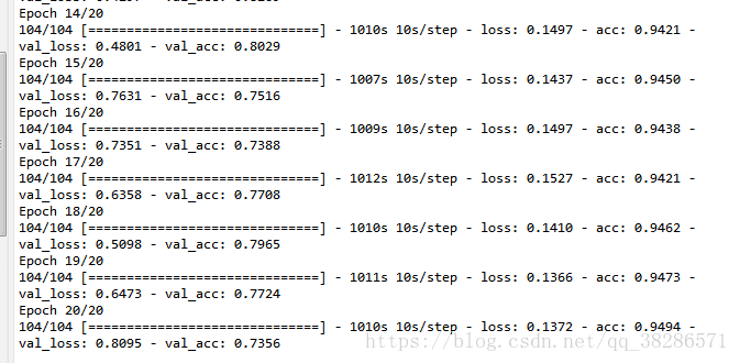
随着迭代次数的增加,loss也逐渐减小,acc也逐渐增大,使用plt模块画图,能更直观的知道模型accuracy和loss函数的迭代过程和规律。代码如下:
acc = history.history['acc']
val_acc = history.history['val_acc']
loss = history.history['loss']
val_loss = history.history['val_loss']
epochs_range = range(1, epochs + 1)

plt.figure(figsize=(8,4))
plt.plot(epochs_range, acc, label='Train Set')
plt.plot(epochs_range, val_acc, label='Test Set')
plt.legend(loc="best")
plt.xlabel('Epochs')
plt.title('Model Accuracy')
plt.show()

plt.figure(figsize=(8,4))
plt.plot(epochs_range, loss, label='Train Set')
plt.plot(epochs_range, val_loss, label='Test Set')
plt.legend(loc="best")
plt.xlabel('Epochs')
plt.title('Model Loss'))
plt.show()
得到的图像规律变化如下:
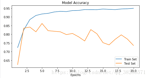
随着训练次数的迭代,model准确率不断上升,第二十步后为0.95,但是随着迭代次数的增加,验证集的准确率在减小。
loss函数变化规律如下:
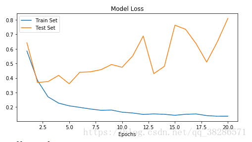
训练集的loss函数值不断减小,但是模型验证集的损失函数却没有变化,甚至有增大的趋势,由此可见,即使在模型中加入了dropout进行优化,也不可避免会有过拟合,出现这种状况的可能与训练集样本过少,而且normal和pneumonia 的样本训练数据数目不一致导致的过拟合。
4、评估模型
评估模型得到相应的准确率(Accuracy),精确率(Precision),召回率(recall);代码如下:
Y_pred = model.predict_generator(test_datagen,test_steps+1)
y_pred = np.argmax(Y_pred,axis=1)
CM =confusion_matrix(test_datagen.classes,y_pred)
print("CM:",CM)

pneumonia_precision= CM[1][1] / (CM[1][0]+CM[1][1])
print("pnuemonia_precision:",pneumonia_precision)
pnuemonia_recall = CM[1][1] / (CM[1][1]+CM[0][1])
print('pnuemonia_recall:',pnuemonia_recall)
accuracy = (CM[0][0]+CM[1][1])/(CM[0][0]+CM[0][1]+CM[1][0]+CM[1][1])

target_names = ['Normal', 'Pneumonia']
print(classification_report(test_datagen.classes, y_pred, target_names=target_names))
输出结果如下:
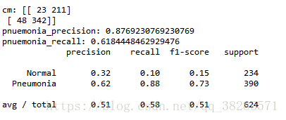
运行文件时accuracy没有加进去,可以根据混淆矩阵CM求出
accuracy=0.5849
根据相应的结果可以知道,模型整体的平均准确率较低,但是模型本身的目的主要是追求Pneumonia的精确率,Pneumonia的精确率达到了0.88。
参考网站:https://www.kaggle.com/paultimothymooney/chest-xray-pneumonia
致谢:
Data:https://data.mendeley.com/datasets/rscbjbr9sj/2
License:CC BY 4.0
Citation:https://www.cell.com/cell/fulltext/S0092-8674(18)30154-5