利用matlab绘制傅里叶分解三维图

版权声明：本文为博主原创文章，未经博主允许不得转载。 https://blog.csdn.net/Stynis/article/details/80531168

目的：

1. 理解傅里叶变换分析及其他方法的分析。
2. 理解傅里叶变换频域与时域的关系。
3. 利用MATLAB绘制傅里叶变换图形三维图。

内容和原理：

本次主要使用的函数及其说明如下（此处只取采用用法的意义说明）：
1.abs：abs(X) is the absolute value of the elements of X. When
X is complex, abs(X) is the complex modulus (magnitude) of
the elements of X.
2.figure: figure, by itself, creates a new figure window, and returns
its handle.
3.square: square(T) generates a square wave with period 2*Pi for the
elements of time vector T. square(T) is like SIN(T), only
it creates a square wave with peaks of +1 to -1 instead of
a sine wave.
4. Fft: fft(X,N) is the N-point fft, padded with zeros if X has less
than N points and truncated if it has more.
5. plot3：plot3(x,y,z), where x, y and z are three vectors of the same length,
plots a line in 3-space through the points whose coordinates are the
elements of x, y and z.

结果与分析：

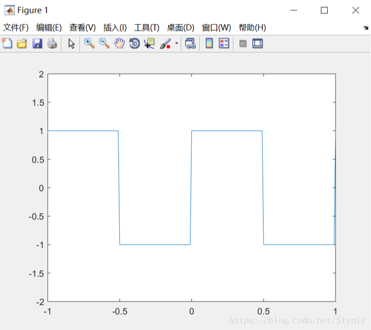
1. 根据要求需要首先产生具有足够采样频率的方波，我采用了square函数生成方波，频率设置为1Hz，采样频率则为100Hz。
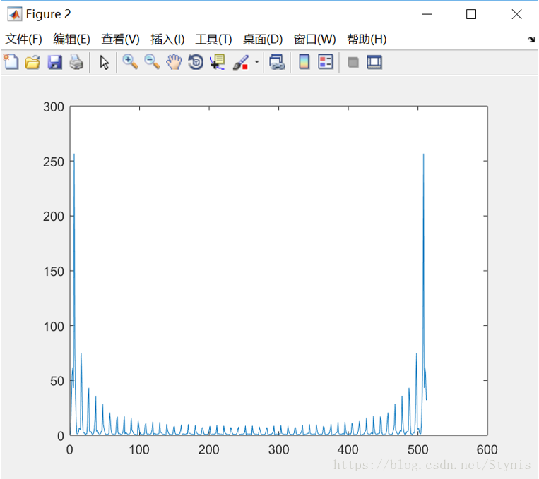
2. 接着进行傅里叶变换，利用fft函数，生成N个分解波形，N越大，分解次数越多，频谱越精密，实验中采用N=512进行实验。
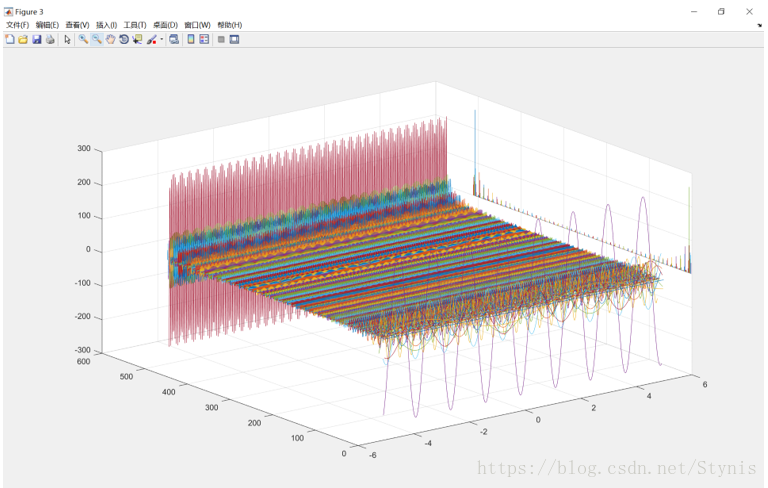
3. 利用plot3函数进行绘图并投影。
   产生的方波图如下：
   
   
   

产生频谱图如下：

绘制三维图像如图：

程序代码如下：

N=512;
fs=100;
t=-2:1/fs:2;
m=square(2*pi*t);  
plot(t,m);
axis([-1 1 -2 2]);
figure();
title('方波');
b=fft(m,N);
mag=abs(b);       
plot(mag);
figure();
x=-5:0.01:5;
for i=1:length(b) 
      for k=1:length(x)
          z(k)=abs(b(i))*sin((i-1)*x(k)+angle(b(i)));
          y(k)=i;
      end
      figure(3);
      grid on;
      plot3(x,y,z);
      hold on;

      x_z=zeros(1,length(x))+6;     
      plot3(x_z,y,abs(z));
      hold on;

end