【 MATLAB 】信号处理工具箱之 fft 案例分析

上篇博文：【 MATLAB 】信号处理工具箱之fft简介及案例分析介绍了MATLAB信号处理工具箱中的信号变换 fft 并分析了一个案例，就是被噪声污染了的信号的频谱分析。

这篇博文继续分析几个小案例：

Gaussian Pulse

这个案例是将高斯脉冲从时域变换到频域，高斯脉冲的信息在下面的程序中都有注释：

clc
clear
close all
% Convert a Gaussian pulse from the time domain to the frequency domain.
% 
% Define signal parameters and a Gaussian pulse, X.

Fs = 100;           % Sampling frequency
t = -0.5:1/Fs:0.5;  % Time vector 
L = length(t);      % Signal length

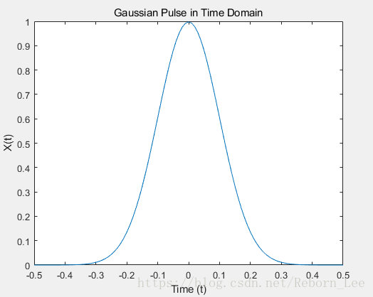
X = 1/(4*sqrt(2*pi*0.01))*(exp(-t.^2/(2*0.01)));
% Plot the pulse in the time domain.
figure();
plot(t,X)
title('Gaussian Pulse in Time Domain')
xlabel('Time (t)')
ylabel('X(t)')

% To use the fft function to convert the signal to the frequency domain, 
% first identify a new input length that is the next power of 2 from the original signal length. 
% This will pad the signal X with trailing zeros in order to improve the performance of fft.

n = 2^nextpow2(L);
% Convert the Gaussian pulse to the frequency domain.
% 
Y = fft(X,n);
% Define the frequency domain and plot the unique frequencies.

f = Fs*(0:(n/2))/n;
P = abs(Y/n);

figure();
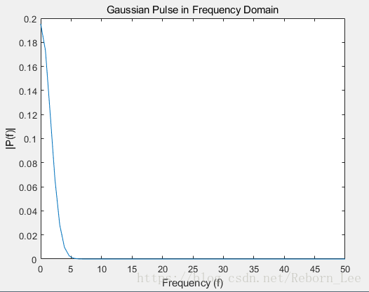
plot(f,P(1:n/2+1)) 
title('Gaussian Pulse in Frequency Domain')
xlabel('Frequency (f)')
ylabel('|P(f)|')

高斯脉冲在时域的图像：

高斯脉冲在频域的图像：

Cosine Waves

这个例子比较简单，就是不同频率的余弦波在时域以及频域的比较：

clc
clear
close all
% Compare cosine waves in the time domain and the frequency domain.
% 
% Specify the parameters of a signal with a sampling frequency of 1kHz and a signal duration of 1 second.

Fs = 1000;                    % Sampling frequency
T = 1/Fs;                     % Sampling period
L = 1000;                     % Length of signal
t = (0:L-1)*T;                % Time vector
% Create a matrix where each row represents a cosine wave with scaled frequency. 
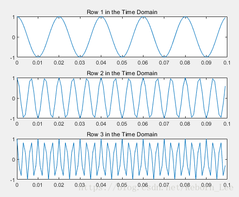
% The result, X, is a 3-by-1000 matrix. The first row has a wave frequency of 50, 
% the second row has a wave frequency of 150, and the third row has a wave frequency of 300.

x1 = cos(2*pi*50*t);          % First row wave
x2 = cos(2*pi*150*t);         % Second row wave
x3 = cos(2*pi*300*t);         % Third row wave

X = [x1; x2; x3];
% Plot the first 100 entries from each row of X in a single figure in order and compare their frequencies.

figure();
for i = 1:3
    subplot(3,1,i)
    plot(t(1:100),X(i,1:100))
    title(['Row ',num2str(i),' in the Time Domain'])
end

% For algorithm performance purposes, fft allows you to pad the input with trailing zeros. 
% In this case, pad each row of X with zeros so that the length of each row is the next higher power of 2 from the current length. 
% Define the new length using the nextpow2 function.

n = 2^nextpow2(L);
% Specify the dim argument to use fft along the rows of X, that is, for each signal.

dim = 2;
% Compute the Fourier transform of the signals.

Y = fft(X,n,dim);
% Calculate the double-sided spectrum and single-sided spectrum of each signal.

P2 = abs(Y/L);
P1 = P2(:,1:n/2+1);
P1(:,2:end-1) = 2*P1(:,2:end-1);
% In the frequency domain, plot the single-sided amplitude spectrum for each row in a single figure.

figure();
for i=1:3
    subplot(3,1,i)
    plot(0:(Fs/n):(Fs/2-Fs/n),P1(i,1:n/2))
    title(['Row ',num2str(i),' in the Frequency Domain'])
end

下图是频率为50Hz，150Hz以及300Hz的余弦波在时域的图像：

下图分别为其fft：

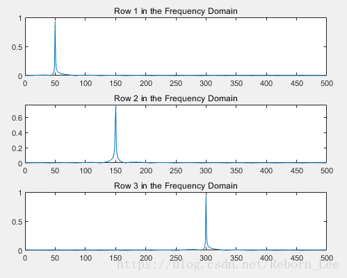
从频域图中可以清晰的看到它们的频率成分位于何处。

【 MATLAB 】信号处理工具箱之 fft 案例分析

Gaussian Pulse

Cosine Waves

猜你喜欢