【 MATLAB 】信号处理工具箱之fft简介及案例分析

clc
clear
close all
% Use Fourier transforms to find the frequency components of a signal buried in noise.
% Specify the parameters of a signal with a sampling frequency of 1 kHz and a signal duration of 1.5 seconds.

Fs = 1000;            % Sampling frequency                    
T = 1/Fs;             % Sampling period       
L = 1500;             % Length of signal
t = (0:L-1)*T;        % Time vector

% Form a signal containing a 50 Hz sinusoid of amplitude 0.7 and a 120 Hz sinusoid of amplitude 1.

S = 0.7*sin(2*pi*50*t) + sin(2*pi*120*t);
% Corrupt the signal with zero-mean white noise with a variance of 4.

X = S + 2*randn(size(t));
 
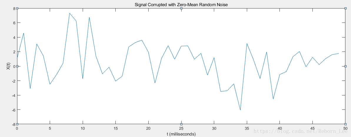
% Plot the noisy signal in the time domain. It is difficult to identify the frequency components by looking at the signal X(t).
figure();
plot(1000*t(1:50),X(1:50))
title('Signal Corrupted with Zero-Mean Random Noise')
xlabel('t (milliseconds)')
ylabel('X(t)')

% Compute the Fourier transform of the signal.
Y = fft(X);

% Compute the two-sided spectrum P2. Then compute the single-sided spectrum P1 based on P2 and the even-valued signal length L.
P2 = abs(Y/L);
P1 = P2(1:L/2+1);
P1(2:end-1) = 2*P1(2:end-1);

% Define the frequency domain f and plot the single-sided amplitude spectrum P1. 
% The amplitudes are not exactly at 0.7 and 1, as expected, because of the added noise. On average, 
% longer signals produce better frequency approximations.
figure();
f = Fs*(0:(L/2))/L;
plot(f,P1) 
title('Single-Sided Amplitude Spectrum of X(t)')
xlabel('f (Hz)')
ylabel('|P1(f)|')

% Now, take the Fourier transform of the original, uncorrupted signal and retrieve the exact amplitudes, 0.7 and 1.0.
% 

Y = fft(S);
P2 = abs(Y/L);
P1 = P2(1:L/2+1);
P1(2:end-1) = 2*P1(2:end-1);

figure();
plot(f,P1) 
title('Single-Sided Amplitude Spectrum of S(t)')
xlabel('f (Hz)')
ylabel('|P1(f)|')

figure（1）是加上零均值的随机噪声后的信号时域图形，通过观察这幅图很难辨别其频率成分。