【学习笔记】基本的图像操作和处理

前面刚配置完opencv以及其环境还有IDE，今天就来用它完成原来学习的数字图像处理中的几个基本的操作与处理。
本次作业参照的是《python计算机视觉编程》中第一章基本的图像操作和处理来完成的。本次基本是参照上面所描述来完成的。

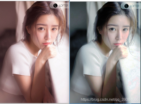
本次仅展示的是以个人的照片为基础实现直方图，高斯滤波以及直方图均衡化的结果。
本次运行时的图片，，找了一张网图。

一 、直方图

通过运行以下代码：

from PIL import Image
from pylab import *

# 添加中文字体支持
from matplotlib.font_manager import FontProperties
font = FontProperties(fname=r"c:\windows\fonts\SimSun.ttc", size=14)
im = array(Image.open('1.jpg').convert('L'))  # 打开图像，并转成灰度图像

figure()
subplot(121)
gray()
contour(im, origin='image')
axis('equal')
axis('off')
title(u'图像轮廓', fontproperties=font)

subplot(122)
hist(im.flatten(), 128)
title(u'图像直方图', fontproperties=font)
plt.xlim([0,260])
plt.ylim([0,11000])

show()

显示结果：

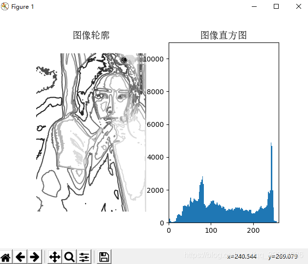
这里使用PIL的convert（）方法将图像转换成灰度图像。

图像的直方图表示该图像像素的分布情况。用一定数目的小区间（bin）来指定表征像素的范围，每个小区间会落到该小区间表示范围的像素数目，该图像的直方图可以使用host（）函数绘制：

figure()
hist(im.flatten(),128)
show()

hist()函数的第二个参数指定小区间的数目。需要注意的是，因为host（）只接受一维数组作为输入，所以我们在绘制图像直方图之前，必须先对图像经行压平处理。flatten（）方法将任意数组按照优先准则转换成一维数组。

二、高斯滤波

高斯模糊可以用于定义图像尺度、计算兴趣点以及很多其他的应用场合。
通过运行下面代码：

from PIL import Image
from pylab import *
from scipy.ndimage import filters

# 添加中文字体支持
from matplotlib.font_manager import FontProperties
font = FontProperties(fname=r"c:\windows\fonts\SimSun.ttc", size=14)

#im = array(Image.open('board.jpeg'))
im = array(Image.open('../data/empire.jpg').convert('L'))

figure()
gray()
axis('off')
subplot(1, 4, 1)
axis('off')
title(u'原图', fontproperties=font)
imshow(im)

for bi, blur in enumerate([2, 5, 10]):
  im2 = zeros(im.shape)
  im2 = filters.gaussian_filter(im, blur)
  im2 = np.uint8(im2)
  imNum=str(blur)
  subplot(1, 4, 2 + bi)
  axis('off')
  title(u'标准差为'+imNum, fontproperties=font)
  imshow(im2)
  show()

可得到下面的高斯模糊结果：

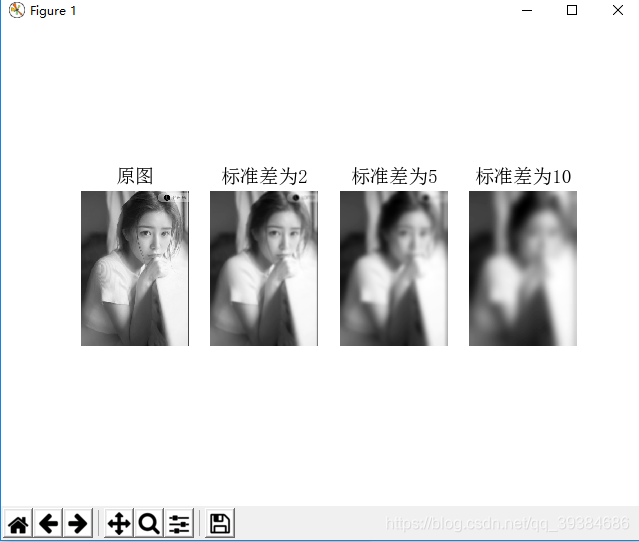
本段代码适用于灰度图像的高斯模糊，如果是处理彩色图像则需要对图像的RGB三个通道经行模糊。

三、直方图均衡化

图像灰度变换中一个非常有用的例子就是直方图的均衡化。直方图的均衡化是指将一副图像的灰度直方图变平，使变换后的图像中每个灰度值的分布概率都相同。在对相同图像做进一步处理之前，直方图均衡化通常是对图像灰度值进行归一化的一个非常好的方法，并且可以增强图像的对比度。
在这种情况下，直方图均衡化的变换函数是图像中像素值的累计分布函数。
运行下面代码：

import cv2 as cv
import numpy as np 
from matplotlib import pyplot as plt


img = cv.imread("1.jpg")
cv.imshow("before", img)

# split g,b,r
g = img[:,:,0]
b = img[:,:,1]
r = img[:,:,2]

# calculate hist
hist_r, bins_r = np.histogram(r, 256)
hist_g, bins_g = np.histogram(g, 256)
hist_b, bins_b = np.histogram(b, 256)

# calculate cdf
cdf_r = hist_r.cumsum()
cdf_g = hist_g.cumsum()
cdf_b = hist_b.cumsum()

# remap cdf to [0,255]
cdf_r = (cdf_r-cdf_r[0])*255/(cdf_r[-1]-1)
cdf_r = cdf_r.astype(np.uint8)# Transform from float64 back to unit8
cdf_g = (cdf_g-cdf_g[0])*255/(cdf_g[-1]-1)
cdf_g = cdf_g.astype(np.uint8)# Transform from float64 back to unit8
cdf_b = (cdf_b-cdf_b[0])*255/(cdf_b[-1]-1)
cdf_b = cdf_b.astype(np.uint8)# Transform from float64 back to unit8

# get pixel by cdf table
r2 = cdf_r[r]
g2 = cdf_g[g]
b2 = cdf_b[b]

# merge g,b,r channel
img2 = img.copy()
img2[:,:,0] = g2
img2[:,:,1] = b2
img2[:,:,2] = r2

# show img after histogram equalization
cv.imshow("img2", img2)

cv.waitKey(0)

可以得到下面的结果：