机械臂——工具标定

版权声明：本文为博主原创文章，遵循 CC 4.0 BY-SA 版权协议，转载请附上原文出处链接和本声明。

本文链接： https://blog.csdn.net/Kalenee/article/details/92591866

一、标定实现

机器人工具坐标系标定就是确定工具坐标系相对于末端连杆坐标系的变换矩阵

1.1 TCP位置标定

标定步骤

1. 控制机械臂移动工具从不同方位触碰空间中某个固定点，记录N组数据（ $n \geqslant 3$）；
2. 计算获得工具末端点相对机械臂末端点的位置变换；

1.2 TCF姿态标定

标定步骤

1. 完成位置标定；
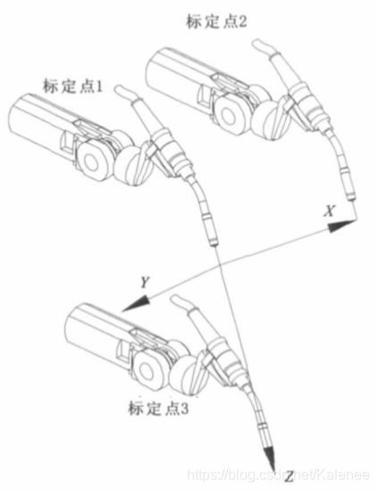
2. 控制工具末端点分别沿x方向和z方向移动一定距离，工具末端点只在该方向上有移动，其它方向上无位移，同时固定初始姿态保持不变。实际操作上可以设置三个固定点（三个固定点满足上述要求，点2和点3相对点1只有一个方向上的移动），使工具末端点分别触碰这三个点然后记录下机械臂末端位姿；
3. 计算获得工具坐标系相对机械臂末端坐标系的姿态变换；

二、原理分析

末端连杆坐标系{E}到基坐标系{B}的位姿关系为：
$_{E}^{B}\textrm{T} = \begin{bmatrix} _{E}^{B}\textrm{R} & _{}^{B}\textrm{p}_{E_0}\\ 0\ 0\ 0 & 1 \end{bmatrix} = \begin{bmatrix} _{E}^{B}\textrm{n}&_{E}^{B}\textrm{o}&_{E}^{B}\textrm{a} & _{}^{B}\textrm{p}_{E_0}\\ 0& 0& 0 & 1 \end{bmatrix} \tag{1}$

$_{E}^{B}\textrm{T}$可通过运动学正解获得， $_{E}^{B}\textrm{R}$为末端连杆坐标系{E}相对于基坐标系{B}的旋转矩阵， $_{}^{B}\textrm{p}_{E_0}$为末端连杆坐标系{E}原点相对于基坐标系{B}的位置矢量。

工具坐标系{T}到基坐标系{B}的位姿关系为：
$_{E}^{B}\textrm{T} \cdot _{T}^{E}\textrm{T} = _{T}^{B}\textrm{T} \tag{2}$

2.1 TCP位置标定分析

在TCP位置标定过程中，第i个标定点的末端连杆坐标系到基坐标系的变换矩阵 $_{E}^{B}\textrm{T}$，可由机器人正解得到，代入\式(2)可得：
$_{E}^{B}\textrm{T}_{i} \cdot _{T}^{E}\textrm{T} = _{T}^{B}\textrm{T}_{i}$
写成分块形式为：
$\begin{bmatrix} _{E}^{B}\textrm{R}_{i} & _{}^{B}\textrm{p}_{{iE}_o}\\ 0\ 0\ 0 & 1 \end{bmatrix} \cdot \begin{bmatrix} _{T}^{E}\textrm{R} & _{}^{B}\textrm{p}_{tcp}\\ 0\ 0\ 0 & 1 \end{bmatrix}= \begin{bmatrix} _{E}^{B}\textrm{R}_{i} & _{}^{B}\textrm{p}_{tcp}\\ 0\ 0\ 0 & 1 \end{bmatrix} \tag{3}$
令等式两边第4列对应相等，则得：
$_{E}^{B}\textrm{R}_{i} \cdot _{}^{B}\textrm{p}_{tcp} + _{}^{B}\textrm{p}_{{iE}_o} = _{}^{B}\textrm{p}_{tcp}$
因工作坐标系{T}相对末端连杆坐标系{E}的位置关系为固定，因此$ {}^{B}\textrm{p}{tcp}$为确定值。所以，对于所有标定点有如下关系：

$\begin{aligned} _{E}^{B}\textrm{R}_{1} \cdot _{}^{B}\textrm{p}_{tcp} + _{}^{B}\textrm{p}_{{iE}_0}&= _{E}^{B}\textrm{R}_{2} \cdot _{}^{B}\textrm{p}_{tcp} + _{}^{B}\textrm{p}_{{iE}_o}\\ &=\cdots\\ &= _{E}^{B}\textrm{R}_{n} \cdot _{}^{B}\textrm{p}_{tcp} + _{}^{B}\textrm{p}_{{iE}_o} \end{aligned}$

写成矩阵形式：

$\begin{bmatrix} _{E}^{B}\textrm{R}_{1} - _{E}^{B}\textrm{R}_{2}\\ _{E}^{B}\textrm{R}_{2} - _{E}^{B}\textrm{R}_{3}\\ \vdots \\ _{E}^{B}\textrm{R}_{n-1} - _{E}^{B}\textrm{R}_{n} \end{bmatrix} \cdot _{}^{E}\textrm{p}_{tcp} =\begin{bmatrix} _{}^{B}\textrm{P}_{{2}E_0} - _{}^{B}\textrm{P}_{{1}E_o}\\ _{}^{B}\textrm{P}_{{3}E_0} - _{}^{B}\textrm{P}_{{2}E_o}\\ \vdots \\ _{}^{B}\textrm{P}_{{n}E_0} - _{}^{B}\textrm{P}_{{n-1}E_o}\\ \end{bmatrix} \tag{4}$

上式的未知量 $_{}^{E}\textrm{p}_{tcp}$含三个元素，包含 $3(n-1)$个方程，系数矩阵为 $3(n-1) \times 3$矩阵。

当 $n \geqslant 3$时系数矩阵秩一般等于3，为列满秩矩阵，式(4)为不相容方程组，只能求最佳最小二乘解。

$_{}^{E}\textrm{p}_{tcp} =A^+ \cdot \begin{bmatrix} _{}^{B}\textrm{P}_{{2}E_o} - _{}^{B}\textrm{P}_{{1}E_o}\\ _{}^{B}\textrm{P}_{{3}E_o} - _{}^{B}\textrm{P}_{{2}E_o}\\ \vdots \\ _{}^{B}\textrm{P}_{{n}E_o} - _{}^{B}\textrm{P}_{{n-1}E_o}\\ \end{bmatrix}$

非奇异的"方阵"才能叫"可逆矩阵"，奇异的"方阵"叫"不可逆矩阵"。

现代应用中为了解决各种线性方程组(系数矩阵是非方阵和方阵为奇异)，将逆矩阵的概念推广到"不可逆方阵"和"长方形矩阵"上，从而产生了"广义逆矩阵"的概念

若A为行满秩，则 $A^+ = A^H(AA^H)^{-1}$

若A为列满秩，则 $A^+ = (A^{H}A)^{-1}A^H$

$A^+$为系数矩阵的加号广义逆，因系数矩阵为列满秩，满足 $A^+ = (A^{H}A)^{-1}A^H$，则：

$_{}^{E}\textrm{p}_{tcp}= \begin{bmatrix} \begin{bmatrix} _{E}^{B}\textrm{R}_{1} - _{E}^{B}\textrm{R}_{2}\\ _{E}^{B}\textrm{R}_{2} - _{E}^{B}\textrm{R}_{3}\\ \vdots \\ _{E}^{B}\textrm{R}_{n-1} - _{E}^{B}\textrm{R}_{n} \end{bmatrix}^{T} \cdot \begin{bmatrix} _{E}^{B}\textrm{R}_{1} - _{E}^{B}\textrm{R}_{2}\\ _{E}^{B}\textrm{R}_{2} - _{E}^{B}\textrm{R}_{3}\\ \vdots \\ _{E}^{B}\textrm{R}_{n-1} - _{E}^{B}\textrm{R}_{n} \end{bmatrix} \end{bmatrix}^{-1} \cdot \begin{bmatrix} _{E}^{B}\textrm{R}_{1} - _{E}^{B}\textrm{R}_{2}\\ _{E}^{B}\textrm{R}_{2} - _{E}^{B}\textrm{R}_{3}\\ \vdots \\ _{E}^{B}\textrm{R}_{n-1} - _{E}^{B}\textrm{R}_{n} \end{bmatrix}^{T} \cdot \begin{bmatrix} _{}^{B}\textrm{P}_{{2}E_o} - _{}^{B}\textrm{P}_{{1}E_o}\\ _{}^{B}\textrm{P}_{{3}E_o} - _{}^{B}\textrm{P}_{{2}E_o}\\ \vdots \\ _{}^{B}\textrm{P}_{{n}E_o} - _{}^{B}\textrm{P}_{{n-1}E_o}\\ \end{bmatrix} \tag{5}$

根据求得的 $_{}^{E}\textrm{p}_{tcp}$可计算标定误差
$\begin{aligned} \delta &= \begin{vmatrix} \begin{bmatrix} _{E}^{B}\textrm{R}_{1} - _{E}^{B}\textrm{R}_{2}\\ _{E}^{B}\textrm{R}_{2} - _{E}^{B}\textrm{R}_{3}\\ \vdots \\ _{E}^{B}\textrm{R}_{n-1} - _{E}^{B}\textrm{R}_{n} \end{bmatrix} \cdot _{}^{E}\textrm{p}_{tcp} - \begin{bmatrix} _{}^{B}\textrm{P}_{{2}E_o} - _{}^{B}\textrm{P}_{{1}E_o}\\ _{}^{B}\textrm{P}_{{3}E_o} - _{}^{B}\textrm{P}_{{2}E_o}\\ \vdots \\ _{}^{B}\textrm{P}_{{n}E_o} - _{}^{B}\textrm{P}_{{n-1}E_o}\\ \end{bmatrix} \end{vmatrix}\\ &=(\sum_{n}^{n-1}|(_{B}^{E}\textrm{R}_{i}- _{B}^{E}\textrm{R}_{i+1}) \cdot _{}^{E}\textrm{P}_{tcp}-_{}^{B}\textrm{P}_{{(i+1)E}_o}+_{}^{B}\textrm{P}_{{iE}_o}|^{2})^{\frac{1}{2}} \end{aligned} \tag{6}$

2.2 TCF姿态标定分析

已知TCF状态标定２个标定点的末端连杆坐标系到基坐标系的变换矩阵，可求得工具中心点相对于基坐标系的位置：

• 中心点和x方向偏移点

$_{}^{B}\textrm{p}_{atcp}= _{E}^{B}\textrm{R}_{o} \cdot _{}^{E}\textrm{p}_{tcp} +_{}^{B}\textrm{p}_{oEo}\\ _{}^{B}\textrm{p}_{xtcp}= _{E}^{B}\textrm{R}_{x} \cdot _{}^{E}\textrm{p}_{tcp} +_{}^{B}\textrm{p}_{xEo}$

• 中心点和z方向偏移点

$_{}^{B}\textrm{p}_{ztcp}= _{E}^{B}\textrm{R}_{z} \cdot _{}^{E}\textrm{p}_{tcp} +_{}^{B}\textrm{p}_{zEo}$

这两点所决定的向量为：
$_{}^{X}\textrm{v}_{} = _{}^{B}\textrm{p}_{xtcp} - _{}^{B}\textrm{p}_{atcp}\\ _{}^{Z}\textrm{v}_{} = _{}^{B}\textrm{p}_{ztcp} - _{}^{B}\textrm{p}_{atcp} \tag{7}$
$_{}^{X}\textrm{v}_{}$为x方向标定点处工具坐标系在+X方向上的向量，即：
$_{}^{X}\textrm{v}_{} = \triangle x \cdot _{E}^{B}\textrm{R}_{o} \cdot _{T}^{E}\textrm{n}_{} \tag{8}$
x轴相对于末端连杆坐标系{E}的方向余弦为：
$_{T}^{E}\textrm{n}_{} = \frac{_{E}^{B}\textrm{R}_{o}^{-1} \cdot (_{E}^{B}\textrm{R}_{x} \cdot _{}^{E}\textrm{p}_{tcp} - _{E}^{B}\textrm{R}_{o} \cdot _{}^{E}\textrm{p}_{tcp} + _{}^{B}\textrm{p}_{xEo} - _{}^{B}\textrm{p}_{oEo})}{|_{E}^{B}\textrm{R}_{x} \cdot _{}^{E}\textrm{p}_{tcp} - _{E}^{B}\textrm{R}_{o} \cdot _{}^{E}\textrm{p}_{tcp} + _{}^{B}\textrm{p}_{xEo} - _{}^{B}\textrm{p}_{oEo}|} \tag{9}$
$_{}^{Z}\textrm{v}_{}$为z方向标定点处工具坐标系在+Z方向上的向量，z轴相对于末端连杆坐标系{E}的方向余弦为：
$_{T}^{E}\textrm{a}_{} = \frac{_{E}^{B}\textrm{R}_{o}^{-1} \cdot (_{E}^{B}\textrm{R}_{z} \cdot _{}^{E}\textrm{p}_{tcp} - _{E}^{B}\textrm{R}_{o} \cdot _{}^{E}\textrm{p}_{tcp} + _{}^{B}\textrm{p}_{zEo} - _{}^{B}\textrm{p}_{oEo})}{|_{E}^{B}\textrm{R}_{z} \cdot _{}^{E}\textrm{p}_{tcp} - _{E}^{B}\textrm{R}_{o} \cdot _{}^{E}\textrm{p}_{tcp} + _{}^{B}\textrm{p}_{zEo} - _{}^{B}\textrm{p}_{oEo}|} \tag{10}$

工具坐标系{T}的Y轴相对于末端连杆坐标系{E}的方向余弦为：
$_{T}^{E}\textrm{o} = _{T}^{E}\textrm{a}\times_{T}^{E}\textrm{n} \tag{11}$
因x方向和z方向为手动移动确定，无法保证两个方向相互垂直，因此需要对其中一个轴（x或者z）进行修正，确保坐标系主矢量的正交性，此处调整z轴：
$_{T}^{E}\textrm{a} = _{T}^{E}\textrm{n}\times_{T}^{E}\textrm{o} \tag{12}$

三、程序实现

import numpy as np
import pandas as pd
import math
from scipy.spatial.transform import Rotation as R

class tool_cal():
    def __init__(self):
        """
		load data from csv
		tool_points(0~5) : use robot effectors to touch the same points in the world
                      and record the pos 
        tool_poses_tran(0~3):count tanslation
        tool_poses_rot(3~5):count rotation
		"""
        with open("tool_data.csv") as file:
            tool_poses = pd.read_csv(file, header = None)
            tool_poses = np.array(tool_poses)
            
            # cal translation
            self.tran_tran=[]
            self.tran_rotm=[]
            tool_poses_tran = tool_poses[0:4,:]
            for pose in tool_poses_tran:
                # set translation
                self.tran_tran.append(np.array([[pose[0]],[pose[1]],[pose[2]]]))
                
                # set rotation
                r = R.from_euler('xyz', np.array([pose[3], pose[4], pose[5]]), degrees=True)
                self.tran_rotm.append(r.as_dcm())

            tool_tran=self.cal_tran()

            # cal rotation
            self.rot_tran=[]
            self.rot_rotm=[]
            tool_poses_rot = tool_poses[3:6,:]
            for pose in tool_poses_rot:
                # set translation
                self.rot_tran.append(np.array([[pose[0]],[pose[1]],[pose[2]]]))
                
                # set rotation
                r = R.from_euler('xyz', np.array([pose[3], pose[4], pose[5]]), degrees=True)
                self.rot_rotm.append(r.as_dcm())

            tool_rot=self.cal_rotm(tool_tran)

            # get transformation
            tool_T = np.array(np.zeros((4,4)))
            tool_T[0:3,0:3] = tool_rot
            tool_T[0:3,3:] = tool_tran
            tool_T[3:,:] = [0,0,0,1]
            print tool_T

    def cal_tran(self):
        tran_data=[]
        rotm_data=[]
        for i in range(len(self.tran_tran)-1):
            tran_data.append(self.tran_tran[i+1] - self.tran_tran[i])
            rotm_data.append(self.tran_rotm[i] - self.tran_rotm[i+1])
        
        L = np.array(np.zeros((3,3)))
        R = np.array(np.zeros((3,1)))
        for i in range(len(tran_data)):
            L = L + np.dot(rotm_data[i],rotm_data[i])
            R = R + np.dot(rotm_data[i],tran_data[i])

        return np.linalg.inv(L).dot(R)

    def cal_rotm(self, tran):
        # centre
        P_otcp_To_B = np.dot(self.rot_rotm[0],tran)+self.rot_tran[0]

        # cal the dircction vector of x
        P_xtcp_To_B = np.dot(self.rot_rotm[1],tran)+self.rot_tran[1]
        vector_X = P_xtcp_To_B - P_otcp_To_B
        dire_vec_x_o = np.linalg.inv(self.rot_rotm[0]).dot(vector_X) / np.linalg.norm(vector_X)

        # cal the dircction vector of z
        P_ztcp_To_B = np.dot(self.rot_rotm[2],tran)+self.rot_tran[2]
        vector_Z = P_ztcp_To_B - P_otcp_To_B
        dire_vec_z_o = np.linalg.inv(self.rot_rotm[0]).dot(vector_Z) / np.linalg.norm(vector_Z)

        # cal the dircction vector of y
        dire_vec_y_o = np.cross(dire_vec_z_o.T,dire_vec_x_o.T)

        # modify the dircction vector of z 
        dire_vec_z_o = np.cross(dire_vec_x_o.T,dire_vec_y_o)

        # cal rotation matrix
        tool_rot = np.array(np.zeros((3,3)))
        tool_rot[:,0] = dire_vec_x_o.T
        tool_rot[:,1] = dire_vec_y_o
        tool_rot[:,2] = dire_vec_z_o
        return tool_rot

if __name__ == "__main__":
    tool_cal()

参考

机器人工具坐标系TCP标定 四点法原理 与 matlab实现

机器人工具坐标系标定算法研究

广义逆矩阵A+