复变函数和积分变换(Complex Function & Integral Transform I)
复变函数和积分变换(Complex Function & Integral Transform II)
复变函数和积分变换(Complex Function & Integral Transform III)
参考文献:
mooc国防科技大学《复变函数》
王忠仁、张静《工程数学:复变函数和积分变换》
焦红伟、尹景本《复变函数与积分变换》
梁昆淼《数学物理方法》
Fourier 变换
所谓积分变换,就是把某函数类 A 中的函数
f(t) 乘上一个确定的二元函数
k(t,p),然后计算积分
F(p)=∫k(t,p)f(t)dt,这样变成另一个函数类 B 中的函数
F(p) 。这里二元函数
k(t,p)是一个确定的二元函数,通常称为该积分变换的核函数(kernel function),
f(t) 称为象原函数(original image function),
F(p) 称为
f(t)的象函数(image function)。如果取积分核
k(ω,t)=e−iωt,就是著名的Fourier 变换。
Fourier 变换(Fourier Transform)
-
周期函数的Fourier 级数:设
fT(t) 是以T为周期的实值函数,在区间
[−2T,2T]上满足狄利克雷(Dirichlet)条件:
(1)连续或只有有限个第一类间断点;
(2)只有有限个极值点
则
fT(t)在连续点处可以展开成Fourier 级数:
fT(t)=2a0+n=1∑∞(ancosnω0t+bnsinnω0t)(F0) 在间断点处,上式左端为
21[fT(t−)+fT(t+)]
其中
ω0=2π/Tan=T2∫−T/2T/2fT(t)cosnω0tdt(n=0,1,2,⋯)bn=T2∫−T/2T/2fT(t)sinnω0tdt(n=1,2,3,⋯)
式 (F0) 称为Fourier 级数的三角形式。
-
Fourier 级数的指数形式:利用欧拉公式
cosθ=2eiθ+e−iθ,sinθ=2ieiθ−e−iθ 将Fourier 级数转化为复指数形式,
fT(t)=c0+n=1∑∞(cneinω0t+c−ne−inω0t)=n=−∞∑∞cneinω0t(F1) 其中
cn=T1∫−T/2T/2fT(t)e−inω0tdt(n=0,±1,±2,⋯)(F2) 由
cn与
an,bn的关系可知
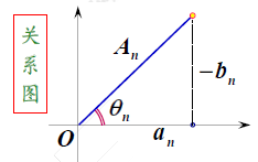
⎩⎪⎨⎪⎧cn=c−n=21an2+bn2
=21Anargcn=−argc−n=θn∣c0∣=A0
-
Fourier 级数的物理含义:
针对Fourier 级数的三角形式 (F0) ,取
A0=a0/2,令
An=an2+bn2
,cosθn=an/An,sinθn=−bn/An,则(F0)化为
fT(t)=A0+n=1∑∞An(cosθncosnω0t+sinθnsinnω0t)=A0+n=1∑∞Ancos(nω0t+θn)
(1) 上式表明,周期信号可以分解为一系列固定频率的简谐波之和,这些简谐波的(角) 频率(frequency) 为一个基频(fundamental frequency)
ω0的倍数。
振幅(amplitude)
An 反映了在信号
fT(t) 中频率为
nω0的简谐波所占有的份额;
相位(phase)
nω0t+θn反映了在信号
fT(t) 中频率为
nω0的简谐波沿时间轴移动的大小,初相位(Initial Phase) 为
θn。
A0表示周期信号在一个周期内的平均值,也叫 直流分量(DC component),
∣A0∣称为直流分量的振幅。
(2) 对于Fourier 级数的复指数形式,我们不难看出
cn作为复数,其模和辐角恰好反应了第 n次谐波的振幅和初相位,
cn是离散频率
nω0的函数,描述了各次谐波的振幅和初相位随离散频率变化的分布情况。称
cn为
fT(t)的离散频谱(spectrum),
∣cn∣为离散振幅谱(amplitude spectrum),
argcn为离散相位谱(phase spectrum)。
-
非周期函数的Fourier 变换
上面研究的是周期函数,事实上对于一个非周期函数
f(t) 可以看成是一个周期为 T的函数
fT(t) 当
T→+∞时转化而来。
由Fourier 级数式(F1)和式(F2)有
f(t)=T→+∞limn=−∞∑∞[T1∫−T/2T/2fT(τ)e−inω0τdτ]einω0t
记
ωn=nω0,间隔
ω0=Δω,当n 取一切整数时,
ωn 所对应的点便均匀地分布在整个数轴上,并由
T=ω02π=Δω2π 得
f(t)=2π1Δω→0limn=−∞∑∞[∫−π/Δωπ/ΔωfT(τ)e−iωnτdτ]eiωntΔω
这是一个和式得极限,按照积分的定义,在一定条件下,上式可写成
f(t)=2π1∫−∞+∞[∫−∞+∞f(τ)e−iωτdτ]eiωtdω(F3) 这个公式称为函数
f(t)的Fourier 积分公式。应该指出,上式只是由式(F1)的右端从形式上推出来的,是不严格的.。至于一个非周期函数
f(t)在什么条件下,可以用Fourier 积分公式表示,有下面的定理。
Fourier 积分定理:若
f(t)在
R上满足:
(1) 在任一有限区间上满足狄利克雷(Dirichlet)条件;
(2) 在无限区间
(−∞,+∞)上绝对可积 ( 即
∫−∞+∞∣f(t)∣dt 收敛)
则有(F3)式成立
在间断点处,(F3)式左端为
21[f(t−)+f(t+)]
Fourier 变换:如果函数
f(t)满足Fourier 积分定理,由式(F3),令
F(ω)=∫−∞+∞f(τ)e−iωτdτ(F4) 则有
f(t)=2π1∫−∞+∞F(ω)eiωtdω(F5) 从上面两式可以看出,
f(t)和
F(ω)通过确定的积分运算可以互相转换。
(1) (F4)式称为
f(t) Fourier 变换(Fourier transform),记为
F(ω)=F[f(t)] ;
(2) (F5)式称为
F(ω) Fourier 逆变换(inverse Fourier transform),记为
f(t)=F−1[F(ω)] ;
(3)
F(ω)称为
f(t)的象函数(image function),
f(t)称为
F(ω)的象原函数(original image function)。通常称
f(t)与
F(ω)构成一个Fourier 变换对(transform pair),记作
f(t)↔F(ω)
-
Fourier 变换的物理意义
Fourier 积分公式表明非周期函数的频谱是连续取值的。
像函数
F(ω)反映的是函数
f(t)中各频率分量的分布密度,它为复值函数,故可表示为
F(ω)=∣F(ω)∣eiargF(ω)
称
F(ω)为
f(t)的频谱(spectrum),
∣F(ω)∣为振幅谱(amplitude spectrum),
argF(ω)为相位谱(phase spectrum)。
不难证明当
f(t)为实函数时,
∣F(ω)∣为偶函数,
argF(ω)为奇函数。
Fourier 变换的性质
-
线性性质:
F[αf1(t)+βf2(t)]=αF[f1(t)]+βF[f2(t)]
-
平移性质:设
F(ω)=F[f(t)],则
F[f(t−t0)]=e−iωt0F(ω)
F−1[F(ω−ω0)]=eiω0tf(t)
-
伸缩性质(相似性质):设
F(ω)=F[f(t)],a=0,则
F[f(at)]=∣a∣1F(aω)
-
微分性质:若
∣t∣→+∞limf(k)(t)=0(k=0,1,2,⋯,n−1),则
F[f(n)(t)]=(iω)nF[f(t)]
-
积分性质:设
g(t)=∫−∞tf(t)dt,若
t→+∞limg(t)=0则
F[g(t)]=iω1F[f(t)]
-
帕赛瓦尔(Parseval)等式:设
f1(t),f2(t)均为平方可积函数,即
∫−∞+∞∣fk(t)∣2dt<+∞(k=1,2)
设
F1(ω)=F[f1(t)],F2(ω)=F[f2(t)],则
∫−∞+∞f1(t)f2(t)dt=2π1∫−∞+∞F1(ω)F2(ω)dω
特别的当
f1(t)=f2(t)=f(t),F(ω)=F[f(t)]时
∫−∞+∞∣f(t)∣2dt=2π1∫−∞+∞∣F(ω)∣2dω
平方可积函数在物理上就是能量有限的信号,上式也叫能量积分(energy integral),
∣F(ω)∣2 也叫能量谱密度(energy spectrum density)。
-
卷积定理:设
F1(ω)=F[f1(t)],F2(ω)=F[f2(t)],则有
F[f1∗f2]=F1(ω)⋅F2(ω)F−1[F1(ω)⋅F2(ω)]=f1∗f2
我们还可以得到
F[f1⋅f2]=F1(ω)∗F2(ω)
δ 函数(δ Function)
在数学、物理学以及实际工程技术中,一些常用的函数,如常数函数、线性函数、符号函数以及单位阶跃函数等等,都不能进行Fourier 变换。
在物理学中,常有集中于一点或一瞬时的量,如脉冲力、脉冲电压、点电荷、质点的质量。
只有引入一个特殊函数来表示它们的分布密度,才有可能把这种集中的量与连续分布的量来统一处理。
- 单位脉冲函数(Unit Impulse Function)
<引例>:假设在原来电流为零的电路中,在 t=0 时瞬时进入一电量为
q0的脉冲。现在确定电流强度分布
i(t),分析可知
i(t)={0∞(t=0)(t=0)
同时需要引入积分值表示电量大小
∫−∞+∞i(t)dt=q0
为此我们引入单位脉冲函数,又称为Dirac函数或者δ函数。
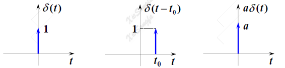
定义:单位脉冲函数
δ(t) 满足
(1) 当
t=0 时,
δ(t)=0
(2)
∫−∞+∞δ(t)dt=1
由此,引例可表示为
i(t)=q0δ(t)
注意:
(1) 单位脉冲函数
δ(t) 并不是经典意义下的函数,因此通常称其为广义函数(或者奇异函数)。
(2) 它不能用常规意义下的值的对应关系来理解和使用,而总是通过它的性质来使用它。
(3) 单位脉冲函数
δ(t) 有多种定义方式,前面所给出的定义方式是由Dirac(狄拉克)给出的。
-
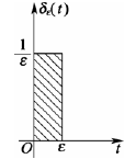
单位脉冲函数其他定义方式
构造一个在 ε时间内激发的矩形脉冲
δε(t),定义为
δε(t)=⎩⎪⎨⎪⎧01/ε0(t<0)(0⩽t⩽ε)(t>ε)
对于任何一个在
R=(−∞,+∞)上无穷次可微的函数
f(t)如果满足
ε→0lim∫−∞+∞δε(t)f(t)dt=∫−∞+∞δ(t)f(t)dt,则称
δε(t)的若极限为
δ(t),记为
ε→0limδε(t)=δ(t)
-
δ函数的性质
筛选性质(sifting property): 设函数
f(t) 是定义在
R上的有界函数,且在
t=0 处连续,则有
∫−∞+∞δ(t)f(t)dt=ε→0limf(θε)=f(0)
更一般的
∫−∞+∞δ(t−t0)f(t)dt=f(t0)
证明:取
f(t)≡1,则有
∫−∞+∞δ(t)dt=ε→0lim∫0εε1dt=1
事实上
∫−∞+∞δ(t)f(t)dt=ε→0lim∫−∞+∞δε(t)f(t)dt=ε→0limε1∫0εf(t)dt
由微分中值定理有
ε1∫0εf(t)dt=f(θε)(0<θ<1)
从而
∫−∞+∞δ(t)f(t)dt=ε→0limf(θε)=f(0)
-
δ函数的另外几条基本性质:(这些性质的严格证明可参阅广义函数)
(1)
δ(t)=δ(−t)
(2)
tδ(t)≡0
(3)
f(t)δ(t−t0)=f(t0)δ(t−t0),f(t)为任意无穷可微函数
(4)
δ(at)=∣a∣1δ(t)(a=0)
(5) 设
u(t)为单位阶跃函数(unit step function),即
u(t)=∫−∞tδ(ξ)dξ={1,0,t>0t<0 则
dtdu(t)=δ(t)
(6)
f(t)∗δ(t)=f(t)
一般的
f(t)∗δ(t−t0)=f(t−t0)
-
δ函数的Fourier 变换:
(1) 根据δ函数筛选性质可得
F(ω)=F[δ(t)]=∫−∞+∞δ(t)e−iωtdt=e−iωt∣t=0=1
δ(t)=F−1[1]=2π1∫−∞+∞eiωtdω
由此可见,单位冲激函数包含所有频率成份,且它们具有相等的幅度,称此为均匀频谱或白色频谱。
可以得到 :
δ(t))↔1δ(t−t0)↔e−iωt01↔2πδ(ω)e−iω0t↔2πδ(ω−ω0)
(2) 有许多重要的函数不满足Fourier 积分定理条件(绝对可积),例如常数、符号函数、单位阶跃函数、正弦函数和余弦函数等,但它们的广义Fourier 变换也是存在的,利用单位脉冲函数及其Fourier 变换可以求出它们的Fourier 变换。
在δ函数的Fourier变换中,其广义积分是根据δ函数的性质直接给出的,而不是按通常的积分方式得到的,称这种方式的Fourier 变换为广义Fourier 变换。
- 周期函数的Fourier 变换
定理:设
f(t) 以T 为周期,在
[0,T] 上满足 Dirichlet 条件,则
f(t)的Fourier 变换为:
F(ω)=2πn=−∞∑+∞F(nω0)δ(ω−nω0) 其中
ω0=2π/T,F(nω0)是
f(t) 的离散频谱。
Fourier 变换的应用(Application of Fourier Transform)
-
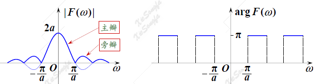
求矩形脉冲函数(rectangular pulse function)
f(t)={10∣t∣<a∣t∣>a 的Fourier 变换及其Fourier 积分表达式。
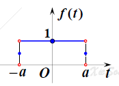
(1) Fourier 变换为
F(ω)=∫−∞+∞f(t)e−iωtdt=∫−aae−iωtdt=∫−aacos(ωt)dt−i∫−aasin(ωt)dt=2∫0acos(ωt)dt=ω2sin(aω)=2aaωsin(aω)
(2) 振幅谱
∣F(ω)∣=2a∣∣∣∣aωsin(aω)∣∣∣∣
相位谱
argF(ω)={0πa2nπ⩽∣ω∣⩽a2nπothers
(3) Fourier 积分表达式为
f(t)=F−1[F(ω)]=2π1∫−∞+∞F(ω)eiωtdω=2π1∫−∞+∞ω2sin(aω)eiωtdω=π1∫−∞+∞ωsin(aω)cosωtdω=⎩⎪⎨⎪⎧1210∣t∣<a∣t∣=a∣t∣>a
在上式中令
t=0,可得重要公式:
∫−∞+∞xsin(ax)dx=⎩⎪⎨⎪⎧−π0πa<0a=0a>0
特别的
∫0+∞xsinxdx=2π
-
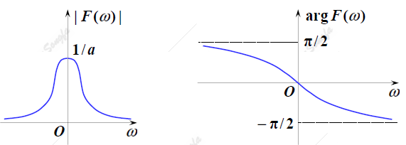
求指数衰减函数(exponential decay function)
f(t)={0e−att<0t⩾0(a>0) 的Fourier 变换及Fourier 积分表达式。
(1) Fourier 变换为
F(ω)=∫−∞+∞f(t)e−iωtdt=∫0+∞e−ate−iωtdt=−(a+iω)1e−(a+iω)t∣∣∣t=0t→+∞=a+iω1=a2+ω2a−iω
(2) 振幅谱
∣F(ω)∣=a2+ω2
1
相位谱
argF(ω)=−arctanaω
(3) Fourier 积分表达式为
f(t)=F−1[F(ω)]=2π1∫−∞+∞F(ω)eiωtdω=2π1∫−∞+∞β2+ω2β−iωeiωtdω=2π1∫−∞+∞β2+ω21(β−iω)(cosωt+isinωt)dω
利用奇偶函数的积分性质,可得
f(t)=π1∫0+∞β2+ω2βcosωt+ωsinωtdω
由此顺便得到一个含参变量广义积分的结果
∫0+∞β2+ω2βcosωt+ωsinωtdω=⎩⎪⎪⎨⎪⎪⎧02ππe−βtt<0t=0t>0
-
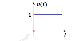
求单位阶跃函数(unit step function)
u(t)={01t<0t>0 的Fourier 变换及其积分表达式。
(1) 现将
u(t)看作是指数衰减函数
f(t;β)={0e−βtt<0t>0 在
β→0+时的极限,即
u(t)=β→0+limf(t;β)
F(ω)=β→0+limF[f(t;β)]=β→0+limβ+iω1=β→0+lim(β2+ω2β−iβ2+ω2ω)=πδ(ω)+iω1
又因
β→0+lim∫−∞+∞β2+ω2βdω=β→0+lim[arctanβω]∣∣∣+∞−∞=π
所以
β→0+limβ2+ω2β=πδ(ω)
F[u(t)]=πδ(ω)+iω1
(2) Fourier 积分表达式
u(t)=F−1[F(ω)]=2π1∫−∞+∞F(ω)eiωtdω=2π1∫−∞+∞[πδ(ω)+iω1]eiωtdω=21∫−∞+∞δ(ω)eiωtdω+2π1∫−∞+∞iω1eiωtdω=21+π1∫0+∞ωsinωtdω
在上式中令 t=1,可得狄利克雷积分
∫0+∞tsintdt=2π
-
求余弦函数
f(t)=cosω0t 的Fourier 积分
由欧拉公式
cosω0t=21(eiω0t+e−iω0t) 有
F[cosω0t]=∫−∞+∞cosω0te−iωtdt=∫0+∞21(eiω0t+e−iω0t)e−iωtdt=21[∫0+∞e−i(ω−ω0)tdt+∫0+∞e−i(ω+ω0)tdt]=π[δ(ω−ω0)+δ(ω+ω0)]
同理可证
F[sinω0t]=iπ[δ(ω+ω0)−δ(ω−ω0)]
Laplace 变换
Laplace 变换(Laplace Transform)
- Fourier 变换的局限性
当函数满足Dirichlet条件,且在
(−∞,+∞) 上绝对可积时,则可以进行古典Fourier 变换。
引入广义函数和广义Fourier 变换是扩大Fourier 变换使用范围的一种方法,却要求有一系列更深刻的数学理论支持。对于以指数级增长的函数,如
eat(a>0) 等,广义Fourier 变换仍无能为力。
如何对Fourier 变换进行改造?
(1) 由于单位阶跃函数
u(t)≡0(t<0),因此
f(t)u(t) 可使积分区间从
(−∞,+∞) 变成
[0,+∞);
(2) 另外,函数
e−βt(β>0) 具有衰减性质,对于许多非绝对可积的函数
f(t),总可选择适当大的 β,使
f(t)u(t)e−βt 满足绝对可积的条件。
通过上述处理,就有希望使得函数
f(t)u(t)e−βt 满足Fourier 变换的条件,从而可以进行Fourier 变换。
F[f(t)u(t)e−βt]=∫−∞+∞f(t)u(t)e−βte−iωtdt=∫0+∞f(t)e−(β+iω)tdt
令
s=β+iω 可得
F[f(t)u(t)e−βt]=∫0+∞f(t)e−stdt
用幂级数推导出 “Laplace 变换”
- Laplace变换
Laplace变换:设函数
f(t) 在
t⩾0时有定义,且积分
∫0+∞f(t)e−stdt在复数 s 的某一个区域内收敛,则此积分所确定的函数
F(s)=∫0+∞f(t)e−stdt称为函数
f(t)的Laplace 变换,记为
F(s)=L[f(t)],函数
F(s) 也可称为
f(t)的象函数。
f(t)=L−1[F(s)]称为Laplace 逆变换。
在Laplace 变换中,只要求
f(t)在
[0,+∞) 内有定义即可。为了研究方便,以后总假定在
(−∞,0) 内,
f(t)≡0
Laplace变换存在定理:设函数
f(t)满足
(1) 在
t⩾0的任何有限区间分段连续;
(2) 当
t→+∞时,
f(t)的增长速度不超过某指数函数,即
∃M>0,C⩾0,使得
∣f(t)∣⩽MeCt(t⩾0) 成立。
则
f(t)的Laplace 变换
F(s)在半平面
Re (s)>C上一定存在,且是解析的。
周期函数的Laplace变换:设
f(t)是
[0,+∞) 内以T 为周期的函数,且逐段光滑,则
L[f(t)]=1−e−sT1∫0Tf(t)e−stdt
Laplace变换的性质
-
线性性质:设
F1(s)=L[f1(t)],F2(s)=L[f2(t)]
L[αf1(t)+βf2(t)]=αF1(s)+βF2(s)
L−1[αF1(s)+βF2(s)]=αf1(t)+βf2(t)
-
位移性质:
L[es0tf(t)]=F(s−s0)
-
微分性质:设
F(s)=L[f(t)]
L[f′(t)]=sF(s)−f(0)
L[f(n)(t)]=snF(s)−k=1∑nsn−kf(k−1)(0)
F′(s)=−L[tf(t)]
F(n)(s)=(−1)nL[tnf(t)]
-
积分性质:设
F(s)=L[f(t)]
L[∫0tf(t)dt]=s1F(s)
L[n times
∫0tdt∫0tdt⋯∫0tf(t)dt]=sn1F(s)
L[tf(t)]=∫s∞F(s)ds
L[tnf(t)]=L[n times
∫s∞dt∫s∞dt⋯∫s∞F(s)ds]
-
延迟性质:
if t>0,f(t)=0,then ∀t0>0
L[f(t−t0)]=e−st0F(s)
L−1[e−st0F(s)]=f(t−t0)u(t−t0)
-
卷积定理:设
F1(s)=L[f1(t)],F2(s)=L[f2(t)],则有
L[f1∗f2]=F1(s)⋅F2(s)L−1[F1(s)⋅F2(s)]=f1∗f2
Laplace 逆变换(Inverse Laplace Transform)
-
反演积分公式(inverse integral formula):由于
f(t) 的Laplace 变换
F(s)=F(β+iω)就是
f(t)u(t)e−βt 的Fourier 变换,即
L[f(t)]=F[f(t)u(t)e−βt]=∫−∞+∞f(t)u(t)e−βte−iωtdt
因此,在
f(t)(t>0)的连续点处有
f(t)u(t)e−βt=2π1∫−∞+∞F(β+iω)eiωtdω
等式两边同乘
eβt,并令
s=β+iω 则有
f(t)u(t)=2πi1∫β−iωβ+iωF(s)estds
因此
f(t)=2πi1∫β−iωβ+iωF(s)estds(t>0)
-
利用留数计算反演积分
定理设
F(s) 在复平面内只有有限个孤立奇点
s1,s2,⋯,sn ,实数 β使这些奇点全在半平面
Re(s)<β 内,且
s→∞limF(s)=0 ,则有
f(t)=k=1∑nRes[F(s)est,sk](t>0)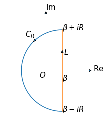
证明:作半圆将所有奇点包围,设
C=CR+L,由于
est在全平面解析,所以
F(s)est的奇点就是
F(s)的奇点,由留数定理可得
2πik=1∑nRes[F(s)est,sk]=∮CF(s)estds=∫β−iRβ+iRF(s)estds+∫CRF(s)estds
由若尔当引理,当 t>0 时,有
R→+∞lim∫CRF(s)estds=0
再根据反演积分公式可得定理公式。
实际中经常遇到有理函数类
F(s)=B(s)A(s),其中
A(s),B(s)是不可约的多项式,当分子
A(s) 的次数小于分母
B(s)的次数时,满足定理对
F(s) 的要求,可用留数计算Laplace 逆变换。
Laplace 变换的应用
常用函数的Laplace变换
-
求指数函数
f(t)=eat(a⩾0)的Laplace 变换
L[eat]=∫0+∞eate−stdt=∫0+∞e−(s−a)tdt
当
Re s>a 时,设
s=β+iω ,此时
t→+∞lime−(s−a)t=t→+∞lime−(β−a)te−iω=0(β>0)
所以有
L[eat]=s−a1(Re s>a)
-
求函数
f(t)=1 的Laplace 变换
L[1]=∫0+∞e−stdt=s1(Re s>0)
-
单位阶跃函数
u(t)={01t<0t>0 的Laplace 变换
L[u(t)]=s1(Re s>0)
-
正弦函数
L[sinωt]=s2+ω2ω(Re s>0)
余弦函数
L[cosωt]=s2+ω2s(Re s>0)
-
幂函数
f(t)=tm(m∈Z+) 的Laplace 变换
L[tm]=∫0+∞tme−stdt=−s1∫0+∞tmde−st=−s1tme−st∣∣∣0+∞+sm∫0+∞tm−1e−stdt=smL[tm−1](Re s>0)
又由
L[1]=1/s,故递推可得
L[tm]=sm+1m!(Re s>0)
-
求 δ 函数的Laplace 变换。
狄利克雷函数
δτ(t)={τ100⩽t<τothers 的Laplace 变换为
L[δτ(t)]=∫0ττ1e−stdt=τs1(1−e−τs)
L[δ(t)]=τ→0limL[δτ(t)]=τ→0limτs1(1−e−τs)
用洛必达法则计算此极限
τ→0limτs1(1−e−τs)=τ→0limsse−τs=1
所以
L[δ(t)]=1
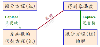
微分方程的Laplace变换解法:主要借助于Laplace变换的微分性质
L[f(n)(t)]=snF(s)−k=1∑nsn−kf(k−1)(0)
(1) 将微分方程(组)化为象函数的代数方程(组);
(2) 求解代数方程得到象函数;
(3) 求Laplace 逆变换得到微分方程(组)的解。
-
求解微分方程
y′′+ω2y=0 满足初始条件
y(0)=0,y′(0)=ω
(1) 令
Y(s)=L[y(t)] ,对方程两边取Laplace 变换
s2Y(s)−sy(0)−y′(0)+ω2Y(s)=0,带入初始条件可得
s2Y(s)−ω+ω2Y(s)=0
(2) 求解此方程,得
Y(s)=s2+ω2ω
(3) 求Laplace 逆变换,得
y=L−1[Y(s)]=sinωt
-
求解微分方程初值问题
{ax′(t)+bx(t)=f(t),x(0)=ct>0
令
X(s)=L[x(t)],F(s)=L[f(t)] ,对方程两边取Laplace 变换,带入初始条件可得
a(sX(s)−c)+bX(s)=F(s)
解得
X(s)=as+bF(s)+ac=cs+b/a1+a1s+b/a1F(s)
由于
L−1[s+b/a1]=e−abt,故上式Laplace 逆变换为
x(t)=ce−abt+a1∫0tf(τ)e−ab(t−τ)dτ
-
求微分方程组:
⎩⎪⎨⎪⎧x′+y+z′=1x+y′+z=0y+4z′=0 满足初始条件
x(0)=0,y(0)=0,z(0)=0
令
L[x(t)]=X(s),L[y(t)]=Y(s),L[z(t)]=Z(s)
对方程组两边取Laplace 变换,并带入初始条件可得
⎩⎪⎪⎨⎪⎪⎧sX(s)+Y(s)+sZ(s)=s1X(s)+sY(s)+Z(s)=0Y(s)+4sZ(s)=0
解代数方程组得:
⎩⎪⎪⎪⎪⎪⎨⎪⎪⎪⎪⎪⎧X(s)=4s2(s2−1)4s2−1Y(s)=s(s2−1)−1Z(s)=4s2(s2−1)1
对每一像函数取Laplace 逆变换可得:
⎩⎪⎪⎪⎪⎨⎪⎪⎪⎪⎧x(t)=L−1[X(s)]=41L−1[s2−13+s21]=41(3sinht+t)y(t)=L−1[Y(s)]=L−1[s1−s2−1s]=1−coshtz(t)=L−1[Z(s)]=41L−1[s2−11−s21]=41(sinht−t)
-
求解积分方程:
f(t)=at−∫0tsin(x−t)f(x)dt(a=0)
原方程化为
f(t)=at+f(t)∗sint
令
F(s)=L[f(t)] ,对方程两边取Laplace 变换
F(s)=s2a+s2+11F(s)
解得
F(s)=a(s2a+s4a)
求Laplace 逆变换
f(t)=a(t+6t3)
物理学问题
-
设质量为m 的物体静止在原点,在 t = 0 时受到 x 方向的冲击力
F0δ(t)的作用,求物体的运动方程。
设物体的运动方程为
x=x(t) ,根据Newton 定律
mx′′(t)=F0δ(t),x(0)=x′(0)=0
令
X(s)=L[x(t)] ,对方程两边取Laplace 变换,并带入初始条件得
ms2X(s)=F0⟹X(s)=ms2F0
求Laplace 逆变换即得物体的运动方程为:
x(t)=mF0t
-
质量为m的物体挂在弹簧系数为k 的弹簧一端(如图),作用在物体上的外力为
f(t)。若物体自静止平衡位置 x = 0 处开始运动,求该物体的运动规律
x(t) 。
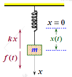
(1) 根据 Newton 定律及 Hooke 定律,物体的运动规律
x(t) 满足如下的微分方程:
mx′′(t)+kx(t)=f(t);x(0)=x′(0)
(2) 令
X(s)=L[x(t)],F(s)=L[f(t)] ,对方程两边取Laplace 变换,带入初始条件可得
ms2X(s)+kX(s)=F(s)
令
ω02=k/m,有
X(s)=mω01⋅s2+ω02ω0⋅F(s)
(3) 利用卷积定理,求Laplace 逆变换得:
x(t)=L−1[X(s)]=mω01[sinω0t∗f(t)]
当
f(t)具体给出时,即可以求得运动规律
x(t)
设物体在 t = 0时受到的外力为
f(t)=Aδ(t)
此时,物体的运动规律为:
x(t)=mω01[sinω0t∗f(t)]=mω0Asinω0t
积分变换附录
|
f(t) |
Fourier Transform |
Laplace Transform |
| Conditions |
若
f(t)在
R上满足:
(1) 在任一有限区间上满足Dirichlet条件;
(2) 在无限区间
(−∞,+∞)上绝对可积 ,即
∫−∞+∞∣f(t)∣dt 收敛
Dirichlet 条件:
(1)连续或只有有限个第一类间断点;
(2)只有有限个极值点 |
若
f(t)满足
(1) 在
t⩾0的任何有限区间分段连续;
(2) 当
t→+∞时,
f(t)的增长速度不超过某指数函数,即
∃M>0,C⩾0,使得
∣f(t)∣⩽MeCt(t⩾0) 成立。
则
f(t)的Laplace 变换
F(s)在半平面
Re (s)>C上一定存在,且是解析的。 |
| Kernel Function |
e−iωt |
e−st |
| Interval |
(−∞,+∞) |
(0,+∞) |
| Symbols |
F(ω)=F[f(t)]
f(t)=F−1[F(ω)] |
F(s)=L[f(t)]
f(t)=L−1[F(s)] |
Transform
(image) |
F(ω)=∫−∞+∞f(τ)e−iωtdt |
F(s)=∫0+∞f(t)e−stdt |
Inverse Transform
(original image) |
f(t)=2π1∫−∞+∞F(ω)eiωtdω |
f(t)=2πi1∫β−iωβ+iωF(s)estds(t>0)
f(t)=k=1∑nRes[F(s)est,sk](t>0) |
Functions
(original image) |
Fourier Transform
(image) |
Laplace Transform |
|
δ(t) |
1 |
1 |
|
δ(t−t0) |
e−iωt0 |
|
| 1 |
2πδ(ω) |
s1(Re s>0) |
|
e−iω0t |
2πδ(ω−ω0) |
|
|
t |
|
s21(Re s>0) |
|
e−at(a⩾0) |
a+iω1 |
s+a1(Re s+a>0) |
|
te−at(a⩾0) |
|
(s+a)21(Re s+a>0) |
|
u(t)={01t<0t>0 |
πδ(ω)+iω1 |
s1(Re s>0) |
|
sgn(t)={−11t<0t>0 |
iω2 |
|
|
rect(t)={10∣t∣<a∣t∣>a |
ω2sin(aω) |
|
|
cosω0t |
π[δ(ω−ω0)+δ(ω+ω0)] |
s2+ω02s(Re s>0) |
|
sinω0t |
iπ[δ(ω+ω0)−δ(ω−ω0)] |
s2+ω02ω0(Re s>0) |
|
tm(m∈Z+) |
|
sm+1m!(Re s>0) |
