【贝叶斯分析③】高斯推断和鲁棒推断

高斯分布是一个非常简单而有用的分布，一方面是因为高斯分布数学上分析起来是否简单。另一个原因可能是中心极限定理（CLT），大致是说当样本数足够多时，样本均值会呈正态分布。

我们可以用高斯分布来对某一观测指标的分布进行建模，高斯分

布的两个参数均值、标准差的先验可以用均匀分布、半正态分布。

# -*- coding: utf-8 -*-

import numpy as np
import pymc3 as pm
import pandas as pd
from scipy import stats
import matplotlib.pyplot as plt
import seaborn as sns


data = np.array([51.06, 55.12, 53.73, 50.24, 52.05, 56.40, 48.45, 52.34, 55.65, 51.49, 51.86, 63.43, 53.00, 56.09, 51.93, 52.31, 52.33, 57.48, 57.44, 55.14, 53.93, 54.62, 56.09, 68.58, 51.36, 55.47, 50.73, 51.94, 54.95, 50.39, 52.91, 51.5, 52.68, 47.72, 49.73, 51.82, 54.99, 52.84, 53.19, 54.52, 51.46, 53.73, 51.61, 49.81, 52.42, 54.3, 53.84, 53.16])


## remove outliers using the interquartile rule# remov 
#quant = np.percentile(data, [25, 75])
#iqr = quant[1] - quant[0]
#upper_b = quant[1] + iqr * 1.5
#lower_b = quant[0] - iqr * 1.5
#clean_data = data[(data > lower_b) & (data < upper_b)]

if __name__ == "__main__":
    
    sns.kdeplot(data)
    plt.xlabel('$x$', fontsize=16)
    
    with pm.Model() as model_g:
        mu = pm.Uniform('mu', lower=40, upper=70)
        sigma = pm.HalfNormal('sigma', sd=10)
        y = pm.Normal('y', mu=mu, sd=sigma, observed=data)
        trace_g = pm.sample(1100, nchains = 1)
        chain_g = trace_g[100:]
        pm.traceplot(chain_g)
        
        plt.figure()
        y_pred = pm.sample_ppc(chain_g, 100, model_g ) #Posterior Predictive Checks，从后验中采样
        sns.kdeplot(data, color='b')
        for i in y_pred['y']:
            sns.kdeplot(i, color='r', alpha=0.1)
        plt.title('Gaussian model', fontsize=16)
        plt.xlabel('$x$', fontsize=16)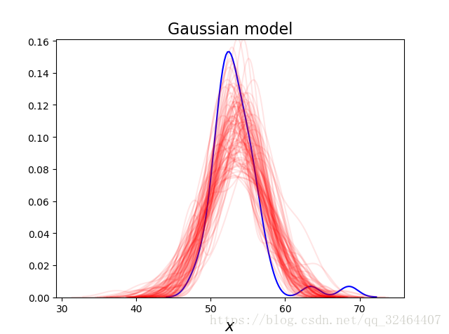

输出结果中，蓝线是data的kde，红线是后验中采样100组的KDE。可以看到采样值的均值要偏右一些，而且采样值的方差也更大。这种现象的原因就是我们的观测数据中有两个点偏离观测数据较远。

为了更好的拟合我们的数据，我们可以更换先验分布来进行鲁棒推断（Robust inferences）。One very useful option when dealing with outliers is to replace the Gaussian likelihood with the Student's t-distribution.和高斯分布相比，t分布有更重的尾部，即偏离均值的数据更有可能出现。另外t分布比高斯分布多了一个参数。

    with pm.Model() as model_t:
        mu = pm.Uniform('mu', 40, 75)
        sigma = pm.HalfNormal('sigma', sd=10)
        nu = pm.Exponential('nu', 1/30)
        y = pm.StudentT('y', mu=mu, sd=sigma, nu=nu, observed=data)
        trace_t = pm.sample(1100)
        
        chain_t = trace_t[100:]
        pm.traceplot(chain_t);
        
        plt.figure()
        y_pred = pm.sample_ppc(chain_t, 100, model_t)
        sns.kdeplot(data, c='b')
        for i in y_pred['y']:
            sns.kdeplot(i, c='r', alpha=0.1)
        plt.xlim(35, 75)
        plt.title("Student's t model", fontsize=16)
        plt.xlabel('$x$', fontsize=16)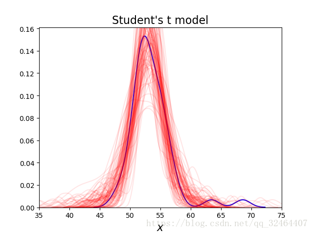

As we can now see, using the Student's t-distribution in our model leads to predictive samples that seem to better fit the data in terms of the location of the peak of the distribution and also its spread;