机器学习 算法基础 五 决策树实践

决策树代码练习例子

---

---

---

代码实践

注意代码安装完py依赖包后还需要安装Graphviz用于生成树结构图

官方windows版本下载链接
然后把 bin默认安装路径C:\Program Files (x86)\Graphviz2.38\bin添加到系统环境变量PATH，重启IDE就可以使用了。

---

练习1：决策树

#!/usr/bin/python
# -*- coding:utf-8 -*-

import numpy as np
import pandas as pd
import matplotlib.pyplot as plt
import matplotlib as mpl
from sklearn import tree
from sklearn.tree import DecisionTreeClassifier
from sklearn.model_selection import train_test_split
from sklearn.pipeline import Pipeline
import pydotplus


# 花萼长度、花萼宽度，花瓣长度，花瓣宽度 （只用了前两个特征）
iris_feature_E = 'sepal length', 'sepal width'#, 'petal length', 'petal width'
iris_feature = u'花萼长度', u'花萼宽度', u'花瓣长度', u'花瓣宽度'
iris_class = 'Iris-setosa', 'Iris-versicolor', 'Iris-virginica'


if __name__ == "__main__":
    mpl.rcParams['font.sans-serif'] = [u'SimHei']
    mpl.rcParams['axes.unicode_minus'] = False

    path = '..\\8.Regression\\iris.data'  # 数据文件路径
    data = pd.read_csv(path, header=None)
    x = data[range(4)]
    y = pd.Categorical(data[4]).codes
    # 为了可视化，仅使用前两列特征
    x = x.iloc[:, :2]
    # 数据集切分为训练集合测试集
    x_train, x_test, y_train, y_test = train_test_split(x, y, train_size=0.7, random_state=1)
    print(y_test.shape)

    # 决策树参数估计
    # min_samples_split = 10：如果该结点包含的样本数目大于10，则(有可能)对其分支
    # min_samples_leaf = 10：若将某结点分支后，得到的每个子结点样本数目都大于10，则完成分支；否则，不进行分支
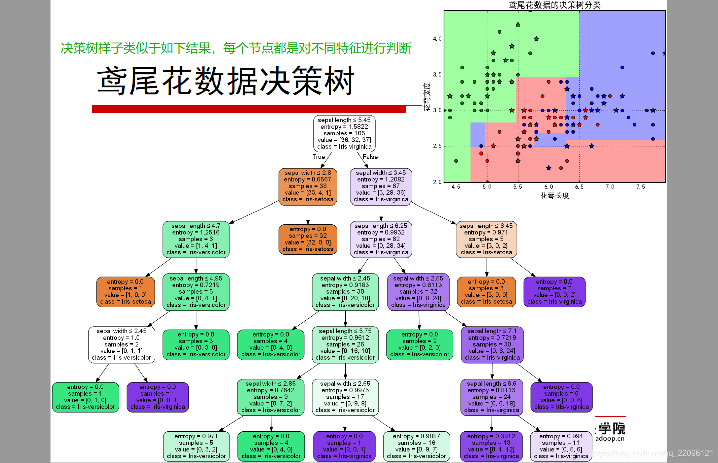
    model = DecisionTreeClassifier(criterion='entropy')
    model.fit(x_train, y_train)
    y_test_hat = model.predict(x_test)      # 测试数据

    # 保存
    # dot -Tpng my.dot -o my.png
    # 1、输出
    with open('iris.dot', 'w') as f:
        tree.export_graphviz(model, out_file=f)
    # 2、给定文件名
    # tree.export_graphviz(model, out_file='iris1.dot')
    # 3、输出为pdf格式
    dot_data = tree.export_graphviz(model, out_file=None, feature_names=iris_feature_E, class_names=iris_class,
                                    filled=True, rounded=True, special_characters=True)
    graph = pydotplus.graph_from_dot_data(dot_data)
    graph.write_pdf('iris.pdf')
    f = open('iris.png', 'wb')
    f.write(graph.create_png())
    f.close()

    # 画图
    N, M = 50, 50  # 横纵各采样多少个值
    x1_min, x2_min = x.min()
    x1_max, x2_max = x.max()
    t1 = np.linspace(x1_min, x1_max, N)
    t2 = np.linspace(x2_min, x2_max, M)
    x1, x2 = np.meshgrid(t1, t2)  # 生成网格采样点
    x_show = np.stack((x1.flat, x2.flat), axis=1)  # 测试点
    print (x_show.shape)

    # # 无意义，只是为了凑另外两个维度
    # # 打开该注释前，确保注释掉x = x[:, :2]
    # x3 = np.ones(x1.size) * np.average(x[:, 2])
    # x4 = np.ones(x1.size) * np.average(x[:, 3])
    # x_test = np.stack((x1.flat, x2.flat, x3, x4), axis=1)  # 测试点

    cm_light = mpl.colors.ListedColormap(['#A0FFA0', '#FFA0A0', '#A0A0FF'])
    cm_dark = mpl.colors.ListedColormap(['g', 'r', 'b'])
    y_show_hat = model.predict(x_show)  # 预测值
    print (y_show_hat.shape)
    print (y_show_hat)
    y_show_hat = y_show_hat.reshape(x1.shape)  # 使之与输入的形状相同
    print (y_show_hat)
    plt.figure(facecolor='w')
    plt.pcolormesh(x1, x2, y_show_hat, cmap=cm_light)  # 预测值的显示
    plt.scatter(x_test[0], x_test[1], c=y_test.ravel(), edgecolors='k', s=150, zorder=10, cmap=cm_dark, marker='*')  # 测试数据
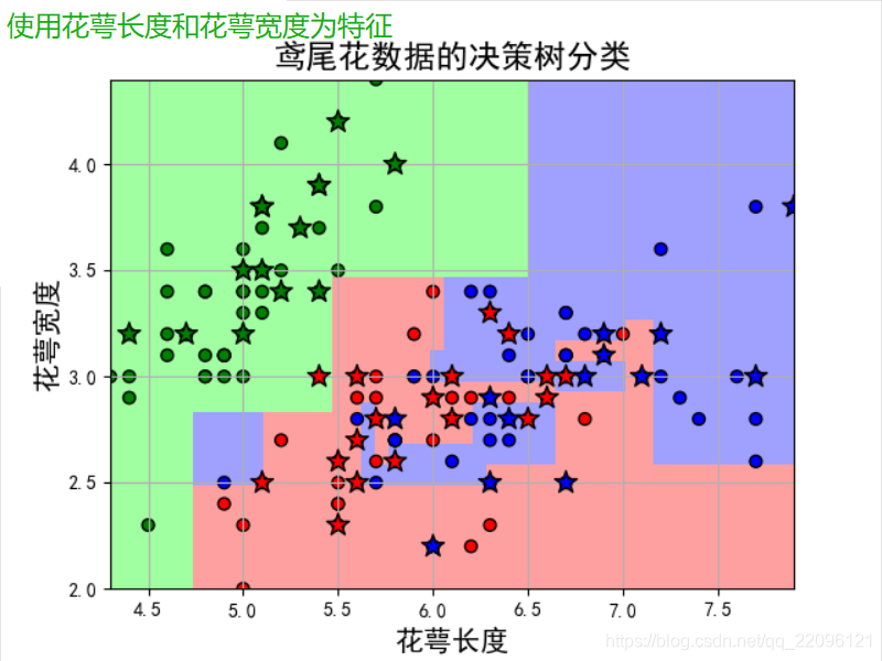
    plt.scatter(x[0], x[1], c=y.ravel(), edgecolors='k', s=40, cmap=cm_dark)  # 全部数据
    plt.xlabel(iris_feature[0], fontsize=15)
    plt.ylabel(iris_feature[1], fontsize=15)
    plt.xlim(x1_min, x1_max)
    plt.ylim(x2_min, x2_max)
    plt.grid(True)
    plt.title(u'鸢尾花数据的决策树分类', fontsize=17)
    plt.show()

    # 训练集上的预测结果
    y_test = y_test.reshape(-1)
    print (y_test_hat)
    print (y_test)
    result = (y_test_hat == y_test)   # True则预测正确，False则预测错误
    acc = np.mean(result)
    print ('准确度: %.2f%%' % (100 * acc))

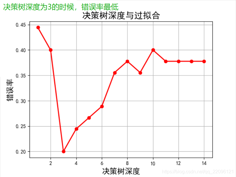
    # 过拟合：错误率
    depth = np.arange(1, 15)
    err_list = []
    for d in depth:
        clf = DecisionTreeClassifier(criterion='entropy', max_depth=d)
        clf.fit(x_train, y_train)
        y_test_hat = clf.predict(x_test)  # 测试数据
        result = (y_test_hat == y_test)  # True则预测正确，False则预测错误
        if d == 1:
            print (result)
        err = 1 - np.mean(result)
        err_list.append(err)
        # print d, ' 准确度: %.2f%%' % (100 * err)
        print (d, ' 错误率: %.2f%%' % (100 * err))
    plt.figure(facecolor='w')
    plt.plot(depth, err_list, 'ro-', lw=2)
    plt.xlabel(u'决策树深度', fontsize=15)
    plt.ylabel(u'错误率', fontsize=15)
    plt.title(u'决策树深度与过拟合', fontsize=17)
    plt.grid(True)
    plt.show()

结果：

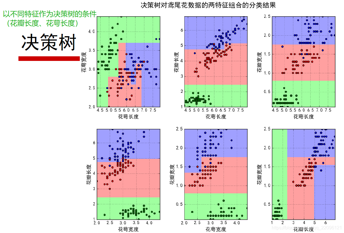
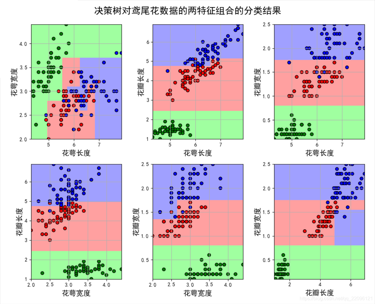
练习2：使用不同的特征组合

#!/usr/bin/python
# -*- coding:utf-8 -*-

import numpy as np
import pandas as pd
import matplotlib as mpl
import matplotlib.pyplot as plt
from sklearn.tree import DecisionTreeClassifier


# 'sepal length', 'sepal width', 'petal length', 'petal width'
iris_feature = u'花萼长度', u'花萼宽度', u'花瓣长度', u'花瓣宽度'

if __name__ == "__main__":
    mpl.rcParams['font.sans-serif'] = [u'SimHei']  # 黑体 FangSong/KaiTi
    mpl.rcParams['axes.unicode_minus'] = False

    path = '..\\8.Regression\\iris.data'  # 数据文件路径
    data = pd.read_csv(path, header=None)
    x_prime = data[range(4)]
    y = pd.Categorical(data[4]).codes

    feature_pairs = [[0, 1], [0, 2], [0, 3], [1, 2], [1, 3], [2, 3]]
    plt.figure(figsize=(10, 9), facecolor='#FFFFFF')
    for i, pair in enumerate(feature_pairs):
        # 准备数据
        x = x_prime[pair]

        # 决策树学习
        clf = DecisionTreeClassifier(criterion='entropy', min_samples_leaf=3)
        clf.fit(x, y)

        # 画图
        N, M = 500, 500  # 横纵各采样多少个值
        x1_min, x2_min = x.min()
        x1_max, x2_max = x.max()
        t1 = np.linspace(x1_min, x1_max, N)
        t2 = np.linspace(x2_min, x2_max, M)
        x1, x2 = np.meshgrid(t1, t2)  # 生成网格采样点
        x_test = np.stack((x1.flat, x2.flat), axis=1)  # 测试点

        # 训练集上的预测结果
        y_hat = clf.predict(x)
        y = y.reshape(-1)
        c = np.count_nonzero(y_hat == y)    # 统计预测正确的个数
        print ('特征：  ', iris_feature[pair[0]], ' + ', iris_feature[pair[1]],)
        print ('\t预测正确数目：', c,)
        print ('\t准确率: %.2f%%' % (100 * float(c) / float(len(y))))

        # 显示
        cm_light = mpl.colors.ListedColormap(['#A0FFA0', '#FFA0A0', '#A0A0FF'])
        cm_dark = mpl.colors.ListedColormap(['g', 'r', 'b'])
        y_hat = clf.predict(x_test)  # 预测值
        y_hat = y_hat.reshape(x1.shape)  # 使之与输入的形状相同
        plt.subplot(2, 3, i+1)
        plt.pcolormesh(x1, x2, y_hat, cmap=cm_light)  # 预测值
        plt.scatter(x[pair[0]], x[pair[1]], c=y, edgecolors='k', cmap=cm_dark)  # 样本
        plt.xlabel(iris_feature[pair[0]], fontsize=14)
        plt.ylabel(iris_feature[pair[1]], fontsize=14)
        plt.xlim(x1_min, x1_max)
        plt.ylim(x2_min, x2_max)
        plt.grid()
    plt.suptitle(u'决策树对鸢尾花数据的两特征组合的分类结果', fontsize=18)
    plt.tight_layout(2)
    plt.subplots_adjust(top=0.92)
    plt.show()

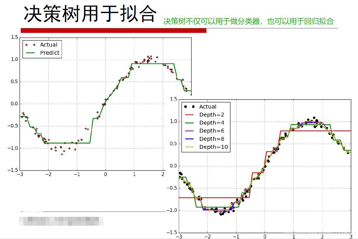
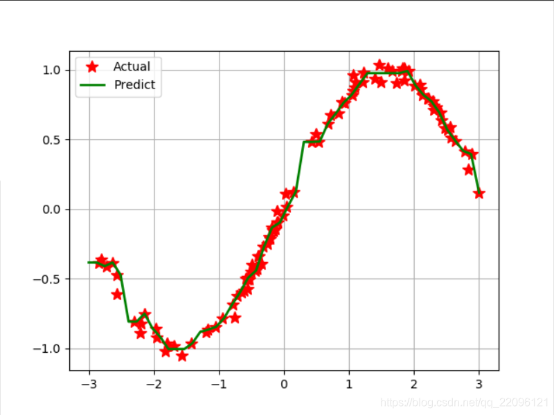
练习3：使用决策树做回归拟合

#!/usr/bin/python
# -*- coding:utf-8 -*-

import numpy as np
import matplotlib.pyplot as plt
from sklearn.tree import DecisionTreeRegressor


if __name__ == "__main__":
    N = 100
    x = np.random.rand(N) * 6 - 3     # [-3,3)
    x.sort()
    y = np.sin(x) + np.random.randn(N) * 0.05
    print (y)
    x = x.reshape(-1, 1)  # 转置后，得到N个样本，每个样本都是1维的
    print( x)

    dt = DecisionTreeRegressor(criterion='mse', max_depth=9)
    dt.fit(x, y)
    x_test = np.linspace(-3, 3, 50).reshape(-1, 1)
    y_hat = dt.predict(x_test)
    plt.plot(x, y, 'r*', ms=10, label='Actual')
    plt.plot(x_test, y_hat, 'g-', linewidth=2, label='Predict')
    plt.legend(loc='upper left')
    plt.grid()
    plt.show()

    # 比较决策树的深度影响
    depth = [2, 4, 6, 8, 10]
    clr = 'rgbmy'
    dtr = DecisionTreeRegressor(criterion='mse')
    plt.plot(x, y, 'ko', ms=6, label='Actual')
    x_test = np.linspace(-3, 3, 50).reshape(-1, 1)
    for d, c in zip(depth, clr):
        dtr.set_params(max_depth=d)
        dtr.fit(x, y)
        y_hat = dtr.predict(x_test)
        plt.plot(x_test, y_hat, '-', color=c, linewidth=2, label='Depth=%d' % d)
    plt.legend(loc='upper left')
    plt.grid(b=True)
    plt.show()

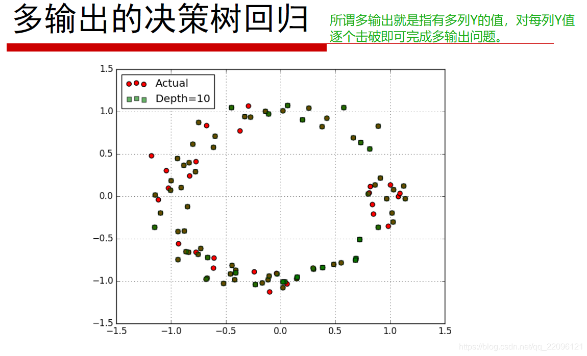
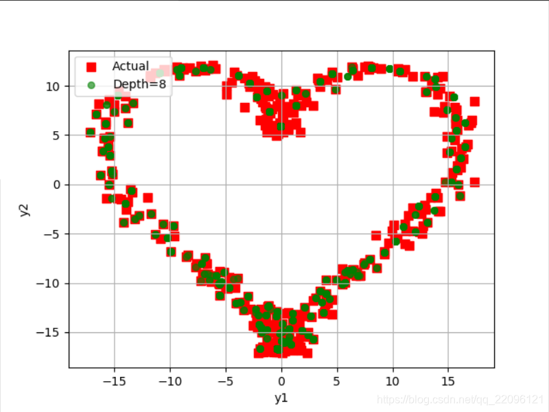
练习4：多输出

#!/usr/bin/python
# -*- coding:utf-8 -*-

import numpy as np
import matplotlib.pyplot as plt
from sklearn.tree import DecisionTreeRegressor


if __name__ == "__main__":
    N = 400
    x = np.random.rand(N) * 8 - 4     # [-4,4)
    x.sort()
    print (x)
    print ('====================')
    # y1 = np.sin(x) + 3 + np.random.randn(N) * 0.1
    # y2 = np.cos(0.3*x) + np.random.randn(N) * 0.01
    # y1 = np.sin(x) + np.random.randn(N) * 0.05
    # y2 = np.cos(x) + np.random.randn(N) * 0.1
    y1 = 16 * np.sin(x) ** 3 + np.random.randn(N)
    y2 = 13 * np.cos(x) - 5 * np.cos(2*x) - 2 * np.cos(3*x) - np.cos(4*x) + 0.1* np.random.randn(N)
    np.set_printoptions(suppress=True)
    print (y1)
    print (y2)
    y = np.vstack((y1, y2)).T
    print (y)
    print ('Data = \n', np.vstack((x, y1, y2)).T)
    print ('=================')
    x = x.reshape(-1, 1)  # 转置后，得到N个样本，每个样本都是1维的

    deep = 8
    reg = DecisionTreeRegressor(criterion='mse', max_depth=deep)
    dt = reg.fit(x, y)

    x_test = np.linspace(-4, 4, num=1000).reshape(-1, 1)
    print (x_test)
    y_hat = dt.predict(x_test)
    print (y_hat)
    plt.scatter(y[:, 0], y[:, 1], c='r', marker='s', s=60, label='Actual')
    plt.scatter(y_hat[:, 0], y_hat[:, 1], c='g', marker='o', edgecolors='g', s=30, label='Depth=%d' % deep, alpha=0.6)
    plt.legend(loc='upper left')
    plt.xlabel('y1')
    plt.ylabel('y2')
    plt.grid()
    plt.show()

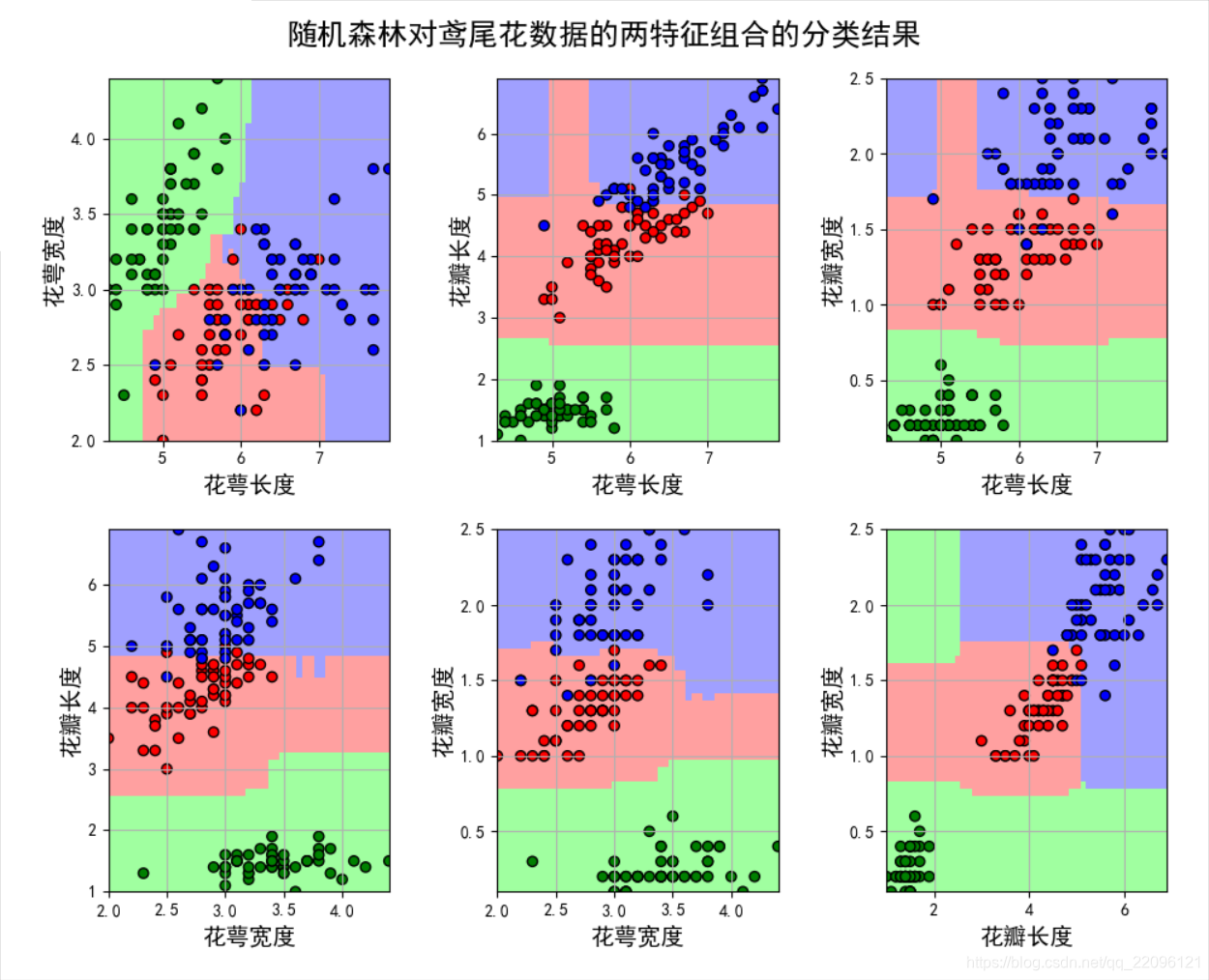
练习5：随机森林对不同特征组合

#!/usr/bin/python
# -*- coding:utf-8 -*-

import numpy as np
import pandas as pd
import matplotlib.pyplot as plt
import matplotlib as mpl
from sklearn.ensemble import RandomForestClassifier


def iris_type(s):
    it = {'Iris-setosa': 0, 'Iris-versicolor': 1, 'Iris-virginica': 2}
    return it[s]

# 'sepal length', 'sepal width', 'petal length', 'petal width'
iris_feature = u'花萼长度', u'花萼宽度', u'花瓣长度', u'花瓣宽度'

if __name__ == "__main__":
    mpl.rcParams['font.sans-serif'] = [u'SimHei']  # 黑体 FangSong/KaiTi
    mpl.rcParams['axes.unicode_minus'] = False

    path = '..\\8.Regression\\iris.data'  # 数据文件路径
    data = pd.read_csv(path, header=None)
    x_prime = data[range(4)]
    y = pd.Categorical(data[4]).codes

    feature_pairs = [[0, 1], [0, 2], [0, 3], [1, 2], [1, 3], [2, 3]]
    plt.figure(figsize=(10, 9), facecolor='#FFFFFF')
    for i, pair in enumerate(feature_pairs):
        # 准备数据
        x = x_prime[pair]

        # 随机森林
        clf = RandomForestClassifier(n_estimators=200, criterion='entropy', max_depth=3)
        clf.fit(x, y.ravel())

        # 画图
        N, M = 50, 50  # 横纵各采样多少个值
        x1_min, x2_min = x.min()
        x1_max, x2_max = x.max()
        t1 = np.linspace(x1_min, x1_max, N)
        t2 = np.linspace(x2_min, x2_max, M)
        x1, x2 = np.meshgrid(t1, t2)  # 生成网格采样点
        x_test = np.stack((x1.flat, x2.flat), axis=1)  # 测试点

        # 训练集上的预测结果
        y_hat = clf.predict(x)
        y = y.reshape(-1)
        c = np.count_nonzero(y_hat == y)    # 统计预测正确的个数
        print ('特征：  ', iris_feature[pair[0]], ' + ', iris_feature[pair[1]],)
        print ('\t预测正确数目：', c,)
        print ('\t准确率: %.2f%%' % (100 * float(c) / float(len(y))))

        # 显示
        cm_light = mpl.colors.ListedColormap(['#A0FFA0', '#FFA0A0', '#A0A0FF'])
        cm_dark = mpl.colors.ListedColormap(['g', 'r', 'b'])
        y_hat = clf.predict(x_test)  # 预测值
        y_hat = y_hat.reshape(x1.shape)  # 使之与输入的形状相同
        plt.subplot(2, 3, i+1)
        plt.pcolormesh(x1, x2, y_hat, cmap=cm_light)  # 预测值
        plt.scatter(x[pair[0]], x[pair[1]], c=y, edgecolors='k', cmap=cm_dark)  # 样本
        plt.xlabel(iris_feature[pair[0]], fontsize=14)
        plt.ylabel(iris_feature[pair[1]], fontsize=14)
        plt.xlim(x1_min, x1_max)
        plt.ylim(x2_min, x2_max)
        plt.grid()
    plt.tight_layout(2.5)
    plt.subplots_adjust(top=0.92)
    plt.suptitle(u'随机森林对鸢尾花数据的两特征组合的分类结果', fontsize=18)
    plt.show()

扫描二维码关注公众号，回复： 9333097 查看本文章

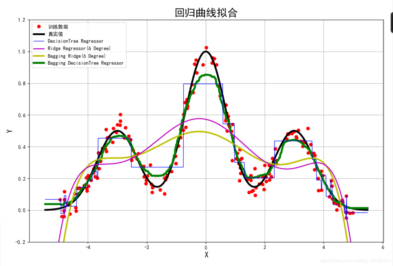
练习6：回归拟合比较

# /usr/bin/python
# -*- encoding:utf-8 -*-

import numpy as np
import matplotlib.pyplot as plt
import matplotlib as mpl
from sklearn.linear_model import RidgeCV
from sklearn.ensemble import BaggingRegressor
from sklearn.tree import DecisionTreeRegressor
from sklearn.pipeline import Pipeline
from sklearn.preprocessing import PolynomialFeatures


def f(x):
    return 0.5*np.exp(-(x+3) **2) + np.exp(-x**2) + 0.5*np.exp(-(x-3) ** 2)


if __name__ == "__main__":
    np.random.seed(0)
    N = 200
    x = np.random.rand(N) * 10 - 5  # [-5,5)
    x = np.sort(x)
    y = f(x) + 0.05*np.random.randn(N)
    x.shape = -1, 1

    degree = 6
    ridge = RidgeCV(alphas=np.logspace(-3, 2, 20), fit_intercept=False)
    ridged = Pipeline([('poly', PolynomialFeatures(degree=degree)), ('Ridge', ridge)])
    bagging_ridged = BaggingRegressor(ridged, n_estimators=100, max_samples=0.2)
    dtr = DecisionTreeRegressor(max_depth=5)
    regs = [
        ('DecisionTree Regressor', dtr),
        ('Ridge Regressor(%d Degree)' % degree, ridged),
        ('Bagging Ridge(%d Degree)' % degree, bagging_ridged),
        ('Bagging DecisionTree Regressor', BaggingRegressor(dtr, n_estimators=100, max_samples=0.2))]
    x_test = np.linspace(1.1*x.min(), 1.1*x.max(), 1000)
    mpl.rcParams['font.sans-serif'] = [u'SimHei']
    mpl.rcParams['axes.unicode_minus'] = False
    plt.figure(figsize=(12, 8), facecolor='w')
    plt.plot(x, y, 'ro', label=u'训练数据')
    plt.plot(x_test, f(x_test), color='k', lw=3.5, label=u'真实值')
    clrs = 'bmyg'
    for i, (name, reg) in enumerate(regs):
        reg.fit(x, y)
        y_test = reg.predict(x_test.reshape(-1, 1))
        plt.plot(x_test, y_test.ravel(), color=clrs[i], lw=i+1, label=name, zorder=6-i)
    plt.legend(loc='upper left')
    plt.xlabel('X', fontsize=15)
    plt.ylabel('Y', fontsize=15)
    plt.title(u'回归曲线拟合', fontsize=21)
    plt.ylim((-0.2, 1.2))
    plt.tight_layout(2)
    plt.grid(True)
    plt.show()