TensorFlow 是一个开源的、基于 Python 的机器学习框架,它由 Google 开发,提供了 Python,C/C++、Java、Go、R 等多种编程语言的接口,并在图形分类、音频处理、推荐系统和自然语言处理等场景下有着丰富的应用,是目前最热门的机器学习框架。
但不少小伙伴跟我吐苦水说Tensorflow的应用太乱了,感觉学的云里雾里,能不能搞个Tensorflow的教程呀。今天,就和大家一起梳理下TensorFlow的十大基础操作。详情如下:
一、Tensorflow的排序与张量
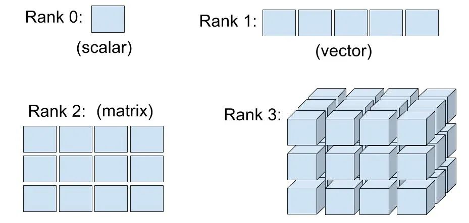
Tensorflow允许用户把张量操作和功能定义为计算图。张量是通用的数学符号,代表保存数据值的多维列阵,张量的维数称为阶。
引用相关的库
import tensorflow as tfimport numpy as np
获取张量的阶(从下面例子看到tf的计算过程)
# 获取张量的阶(从下面例子看到tf的计算过程)g = tf.Graph()# 定义一个计算图with g.as_default(): ## 定义张量t1,t2,t3 t1 = tf.constant(np.pi) t2 = tf.constant([1,2,3,4]) t3 = tf.constant([[1,2],[3,4]]) ## 获取张量的阶 r1 = tf.rank(t1) r2 = tf.rank(t2) r3 = tf.rank(t3) ## 获取他们的shapes s1 = t1.get_shape() s2 = t2.get_shape() s3 = t3.get_shape() print("shapes:",s1,s2,s3)# 启动前面定义的图来进行下一步操作with tf.Session(graph=g) as sess: print("Ranks:",r1.eval(),r2.eval(),r3.eval())

二、Tensorflow 计算图
Tensorflow 的核心在于构建计算图,并用计算图推导从输入到输出的所有张量之间的关系。假设有0阶张量a,b,c,要评估 ,可以表示为下图所示的计算图:
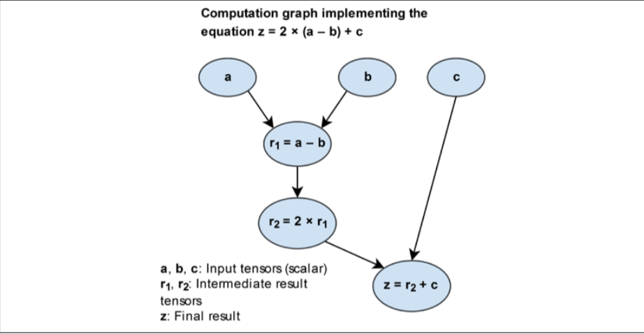
可以看到,计算图就是一个节点网络,每个节点就像是一个操作,将函数应用到输入张量,然后返回0个或者更多个张量作为张量作为输出。
在Tensorflow编制计算图步骤如下:
1. 初始化一个空的计算图
2. 为该计算图加入节点(张量和操作)
3. 执行计算图:
a.开始一个新的会话
b.初始化图中的变量
c.运行会话中的计算图
# 初始化一个空的计算图g = tf.Graph()# 为该计算图加入节点(张量和操作)with g.as_default():a = tf.constant(1,name="a")b = tf.constant(2,name="b")c = tf.constant(3,name="c")z = 2*(a-b)+c# 执行计算图## 通过调用tf.Session产生会话对象,该调用可以接受一个图为参数(这里是g),否则将启动默认的空图## 执行张量操作的用sess.run(),他将返回大小均匀的列表with tf.Session(graph=g) as sess:print('2*(a-b)+c =>',sess.run(z))
2*(a-b)+c => 1
三、Tensorflow中的占位符
Tensorflow有提供数据的特别机制。其中一种机制就是使用占位符,他们是一些预先定义好类型和形状的张量。
通过调用tf.placeholder函数把这些张量加入计算图中,而且他们不包括任何数据。然而一旦执行图中的特定节点就需要提供数据阵列。
3.1 定义占位符
g = tf.Graph()with g.as_default():tf_a = tf.placeholder(tf.int32,shape=(),name="tf_a") # shape=[]就是定义0阶张量,更高阶张量可以用【n1,n2,n3】表示,如shape=(3,4,5)tf_b = tf.placeholder(tf.int32,shape=(),name="tf_b")tf_c = tf.placeholder(tf.int32,shape=(),name="tf_c")r1 = tf_a - tf_br2 = 2*r1z = r2 + tf_c
3.2 为占位符提供数据
当在图中处理节点的时候,需要产生python字典来为占位符来提供数据阵列。
with tf.Session(graph=g) as sess: feed = { tf_a:1, tf_b:2, tf_c:3 } print('z:',sess.run(z,feed_dict=feed))
z: 1
3.3 用batch_sizes为数据阵列定义占位符
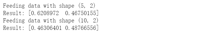
在研发神经网络模型的时候,有时会碰到大小规模不一致的小批量数据。占位符的一个功能是把大小无法确定的维度定义为None。
g = tf.Graph()with g.as_default():tf_x = tf.placeholder(tf.float32,shape=(None,2),name="tf_x")x_mean = tf.reduce_mean(tf_x,axis=0,name="mean")np.random.seed(123)with tf.Session(graph=g) as sess:x1 = np.random.uniform(low=0,high=1,size=(5,2))print("Feeding data with shape",x1.shape)print("Result:",sess.run(x_mean,feed_dict={tf_x:x1}))x2 = np.random.uniform(low=0,high=1,size=(10,2))print("Feeding data with shape",x2.shape)print("Result:",sess.run(x_mean,feed_dict={tf_x:x2}))
四、Tensorflow 的变量
就Tensorflow而言,变量是一种特殊类型的张量对象,他允许我们在训练模型阶段,在tensorflow会话中储存和更新模型的参数。
4.1 定义变量
方式1:tf.Variable() 是为新变量创建对象并将其添加到计算图的类。
- 方式2:tf.get_variable()是假设某个变量名在计算图中,可以复用给定变量名的现有值或者不存在则创建新的变量,因此变量名的name非常重要!
无论采用哪种变量定义方式,直到调用tf.Session启动计算图并且在会话中具体运行了初始化操作后才设置初始值。事实上,只有初始化Tensorflow的变量之后才会为计算图分配内存。
g1 = tf.Graph()with g1.as_default():w = tf.Variable(np.array([[1,2,3,4],[5,6,7,8]]),name="w")print(w)

4.2 初始化变量
由于变量是直到调用tf.Session启动计算图并且在会话中具体运行了初始化操作后才设置初始值,只有初始化Tensorflow的变量之后才会为计算图分配内存。因此这个初始化的过程十分重要,这个初始化过程包括:为 相关张量分配内存空间并为其赋予初始值。
初始化方式:
方式1.tf.global_variables_initializer函数,返回初始化所有计算图中现存的变量,要注意的是:定义变量一定要造初始化之前,不然会报错!!!
方式2:将tf.global_variables_initializer函数储存在init_op(名字不唯一,自己定)对象内,然后用sess.run出来
with tf.Session(graph=g1) as sess: sess.run(tf.global_variables_initializer()) print(sess.run(w))
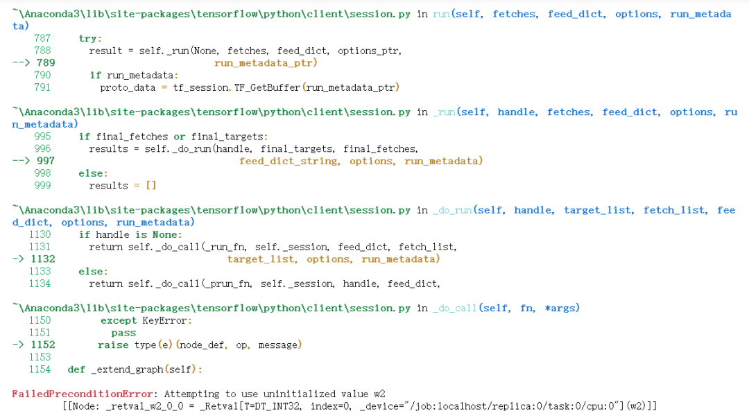
# 我们来比较定义变量与初始化顺序的关系g2 = tf.Graph()with g2.as_default():w1 = tf.Variable(1,name="w1")init_op = tf.global_variables_initializer()w2 = tf.Variable(2,name="w2")with tf.Session(graph=g2) as sess:sess.run(init_op)print("w1:",sess.run(w1))
w1: 1
with tf.Session(graph=g2) as sess: sess.run(init_op) print("w2:",sess.run(w2))
4.3 变量范围
变量范围是一个重要的概念,对建设大型神经网络计算图特别有用。
可以把变量的域划分为独立的子部分。在创建变量时,该域内创建的操作与张量的名字都以域名为前缀,而且这些域可以嵌套。
g = tf.Graph()with g.as_default():with tf.variable_scope("net_A"): #定义一个域net_Awith tf.variable_scope("layer-1"): # 在域net_A下再定义一个域layer-1w1 = tf.Variable(tf.random_normal(shape=(10,4)),name="weights") # 该变量定义在net_A/layer-1域下with tf.variable_scope("layer-2"):w2 = tf.Variable(tf.random_normal(shape=(20,10)),name="weights")with tf.variable_scope("net_B"): # 定义一个域net_Bwith tf.variable_scope("layer-2"):w3 = tf.Variable(tf.random_normal(shape=(10,4)),name="weights")print(w1)print(w2)print(w3)

五、建立回归模型
我们需要定义的变量:
1.输入x:占位符tf_x
2.输入y:占位符tf_y
3.模型参数w:定义为变量weight
4.模型参数b:定义为变量bias
5.模型输出 ̂ y^:有操作计算得到
import tensorflow as tfimport numpy as npimport matplotlib.pyplot as plt%matplotlib inlineg = tf.Graph()# 定义计算图with g.as_default():tf.set_random_seed(123)## placeholdertf_x = tf.placeholder(shape=(None),dtype=tf.float32,name="tf_x")tf_y = tf.placeholder(shape=(None),dtype=tf.float32,name="tf_y")## define the variable (model parameters)weight = tf.Variable(tf.random_normal(shape=(1,1),stddev=0.25),name="weight")bias = tf.Variable(0.0,name="bias")## build the modely_hat = tf.add(weight*tf_x,bias,name="y_hat")## compute the costcost = tf.reduce_mean(tf.square(tf_y-y_hat),name="cost")## train the modeloptim = tf.train.GradientDescentOptimizer(learning_rate=0.001)train_op = optim.minimize(cost,name="train_op")
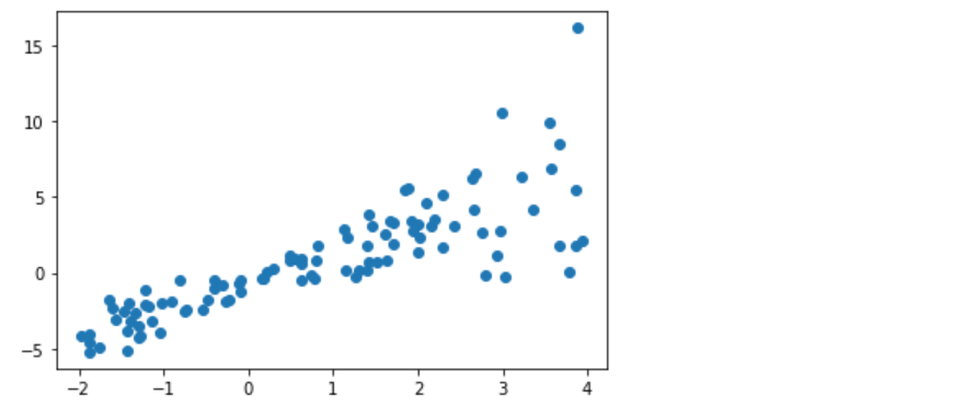
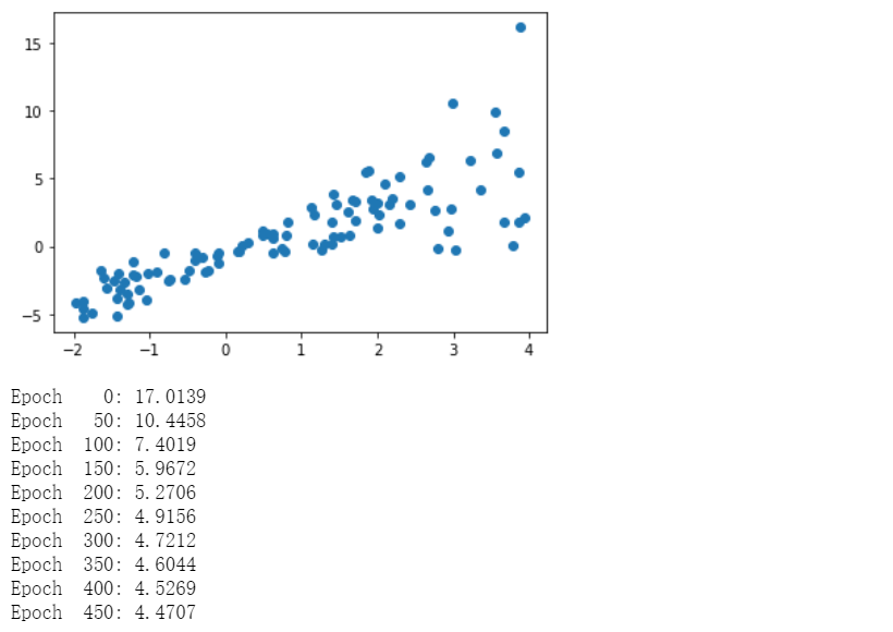
# 创建会话启动计算图并训练模型## create a random toy dataset for regressionnp.random.seed(0)def make_random_data():x = np.random.uniform(low=-2,high=4,size=100)y = []for t in x:r = np.random.normal(loc=0.0,scale=(0.5 + t*t/3),size=None)y.append(r)return x,1.726*x-0.84+np.array(y)x,y = make_random_data()plt.plot(x,y,'o')plt.show()
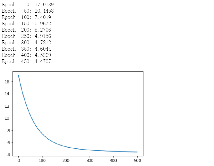
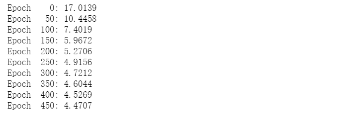
## train/test splitsx_train,y_train = x[:100],y[:100]x_test,y_test = x[100:],y[100:]n_epochs = 500train_costs = []with tf.Session(graph=g) as sess:sess.run(tf.global_variables_initializer())## train the model for n_epochsfor e in range(n_epochs):c,_ = sess.run([cost,train_op],feed_dict={tf_x:x_train,tf_y:y_train})train_costs.append(c)if not e % 50:print("Epoch %4d: %.4f"%(e,c))plt.plot(train_costs)plt.show()
六、在Tensorflow计算图中用张量名执行对象
只需要把
sess.run([cost,train_op],feed_dict={tf_x:x_train,tf_y:y_train})
改为
sess.run(['cost:0','train_op:0'],feed_dict={'tf_x:0':x_train,'tf_y:0':y_train})
注意:只有张量名才有:0后缀,操作是没有:0后缀的,例如train_op并没有train_op:0
## train/test splitsx_train,y_train = x[:100],y[:100]x_test,y_test = x[100:],y[100:]n_epochs = 500train_costs = []with tf.Session(graph=g) as sess:sess.run(tf.global_variables_initializer())## train the model for n_epochsfor e in range(n_epochs):c,_ = sess.run(['cost:0','train_op'],feed_dict={'tf_x:0':x_train,'tf_y:0':y_train})train_costs.append(c)if not e % 50:print("Epoch %4d: %.4f"%(e,c))
七、在Tensorflow中储存和恢复模型
神经网络训练可能需要几天几周的时间,因此我们需要把训练出来的模型储存下来供下次使用。
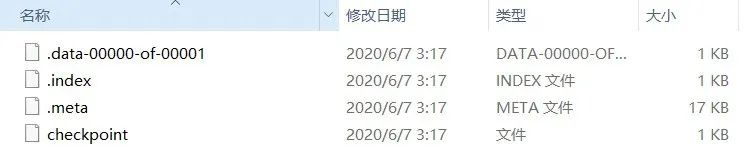
储存的方法是在定义计算图的时候加入:saver = tf.train.Saver(),并且在训练后输入saver.save(sess,'./trained-model')
g = tf.Graph()# 定义计算图with g.as_default():tf.set_random_seed(123)## placeholdertf_x = tf.placeholder(shape=(None),dtype=tf.float32,name="tf_x")tf_y = tf.placeholder(shape=(None),dtype=tf.float32,name="tf_y")## define the variable (model parameters)weight = tf.Variable(tf.random_normal(shape=(1,1),stddev=0.25),name="weight")bias = tf.Variable(0.0,name="bias")## build the modely_hat = tf.add(weight*tf_x,bias,name="y_hat")## compute the costcost = tf.reduce_mean(tf.square(tf_y-y_hat),name="cost")## train the modeloptim = tf.train.GradientDescentOptimizer(learning_rate=0.001)train_op = optim.minimize(cost,name="train_op")saver = tf.train.Saver()# 创建会话启动计算图并训练模型## create a random toy dataset for regressionnp.random.seed(0)def make_random_data():x = np.random.uniform(low=-2,high=4,size=100)y = []for t in x:r = np.random.normal(loc=0.0,scale=(0.5 + t*t/3),size=None)y.append(r)return x,1.726*x-0.84+np.array(y)x,y = make_random_data()plt.plot(x,y,'o')plt.show()## train/test splitsx_train,y_train = x[:100],y[:100]x_test,y_test = x[100:],y[100:]n_epochs = 500train_costs = []with tf.Session(graph=g) as sess:sess.run(tf.global_variables_initializer())## train the model for n_epochsfor e in range(n_epochs):c,_ = sess.run(['cost:0','train_op'],feed_dict={'tf_x:0':x_train,'tf_y:0':y_train})train_costs.append(c)if not e % 50:print("Epoch %4d: %.4f"%(e,c))saver.save(sess,'C:/Users/Leo/Desktop/trained-model/')
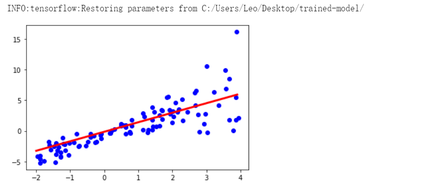
# 加载保存的模型g2 = tf.Graph()with tf.Session(graph=g2) as sess: new_saver = tf.train.import_meta_graph("C:/Users/Leo/Desktop/trained-model/.meta") new_saver.restore(sess,'C:/Users/Leo/Desktop/trained-model/') y_pred = sess.run('y_hat:0',feed_dict={'tf_x:0':x_test})

## 可视化模型x_arr = np.arange(-2,4,0.1)g2 = tf.Graph()with tf.Session(graph=g2) as sess: new_saver = tf.train.import_meta_graph("C:/Users/Leo/Desktop/trained-model/.meta") new_saver.restore(sess,'C:/Users/Leo/Desktop/trained-model/') y_arr = sess.run('y_hat:0',feed_dict={'tf_x:0':x_arr}) plt.figure() plt.plot(x_train,y_train,'bo') plt.plot(x_test,y_test,'bo',alpha=0.3) plt.plot(x_arr,y_arr.T[:,0],'-r',lw=3) plt.show()
八、把张量转换成多维数据阵列
8.1 获得张量的形状
在numpy中我们可以用arr.shape来获得Numpy阵列的形状,而在Tensorflow中则用tf.get_shape函数完成:
注意:在tf.get_shape函数的结果是不可以索引的,需要用as.list()换成列表才能索引。
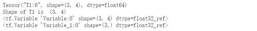
g = tf.Graph()with g.as_default():arr = np.array([[1.,2.,3.,3.5],[4.,5.,6.,6.5],[7.,8.,9.,9.5]])T1 = tf.constant(arr,name="T1")print(T1)s = T1.get_shape()print("Shape of T1 is ",s)T2 = tf.Variable(tf.random_normal(shape=s))print(T2)T3 = tf.Variable(tf.random_normal(shape=(s.as_list()[0],)))print(T3)
8.2 改变张量的形状
现在来看看Tensorflow如何改变张量的形状,在Numpy可以用np.reshape或arr.reshape,在一维的时候可以用-1来自动计算最后的维度。在Tensorflow内调用tf.reshape
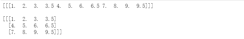
with g.as_default(): T4 = tf.reshape(T1,shape=[1,1,-1],name="T4") print(T4) T5 = tf.reshape(T1,shape=[1,3,-1],name="T5") print(T5)

with tf.Session(graph=g) as sess: print(sess.run(T4)) print() print(sess.run(T5))
8.3 将张量分裂为张量列表
with g.as_default(): tf_splt = tf.split(T5,num_or_size_splits=2,axis=2,name="T8") print(tf_splt)

8.4 张量的拼接
g = tf.Graph()with g.as_default():t1 = tf.ones(shape=(5,1),dtype=tf.float32,name="t1")t2 = tf.zeros(shape=(5,1),dtype=tf.float32,name="t2")print(t1)print(t2)

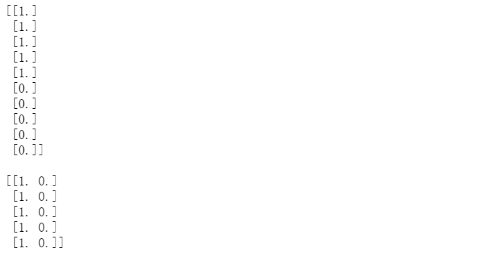
with g.as_default(): t3 = tf.concat([t1,t2],axis=0,name="t3") print(t3) t4 = tf.concat([t1,t2],axis=1,name="t4") print(t4)

with tf.Session(graph=g) as sess: print(t3.eval()) print() print(t4.eval())
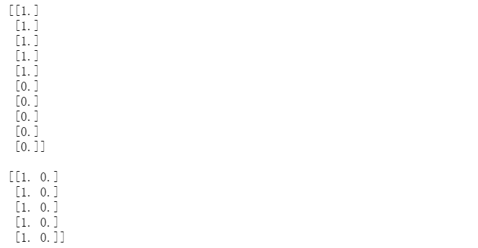
with tf.Session(graph=g) as sess: print(sess.run(t3)) print() print(sess.run(t4))
九、利用控制流构图
这里主要讨论在Tensorflow执行像python一样的if语句,循环while语句,if...else..语句等。
9.1 条件语句tf.cond()语句我们来试试:

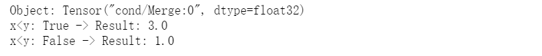
x,y = 1.0,2.0g = tf.Graph()with g.as_default():tf_x = tf.placeholder(dtype=tf.float32,shape=None,name="tf_x")tf_y = tf.placeholder(dtype=tf.float32,shape=None,name="tf_y")res = tf.cond(tf_x<tf_y,lambda: tf.add(tf_x,tf_y,name="result_add"),lambda: tf.subtract(tf_x,tf_y,name="result_sub"))print("Object:",res) #对象被命名为"cond/Merge:0"with tf.Session(graph=g) as sess:print("x<y: %s -> Result:"%(x<y),res.eval(feed_dict={"tf_x:0":x,"tf_y:0":y}))x,y = 2.0,1.0print("x<y: %s -> Result:"%(x<y),res.eval(feed_dict={"tf_x:0":x,"tf_y:0":y}))
9.2 执行python的if...else语句
tf.case()
f1 = lambda: tf.constant(1)f2 = lambda: tf.constant(0)result = tf.case([(tf.less(x,y),f1)],default=f2)print(result)

9.3 执行python的while语句
tf.while_loop()
i = tf.constant(0)threshold = 100c = lambda i: tf.less(i,100)b = lambda i: tf.add(i,1)r = tf.while_loop(cond=c,body=b,loop_vars=[i])print(r)

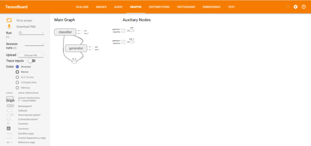
十、用TensorBoard可视化图
TensorBoard是Tensorflow一个非常好的工具,它负责可视化和模型学习。可视化允许我们看到节点之间的连接,探索它们之间的依赖关系,并且在需要的时候进行模型调试。
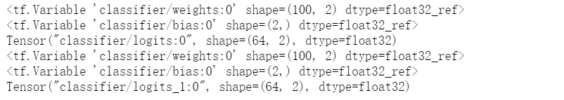
def build_classifier(data, labels, n_classes=2):data_shape = data.get_shape().as_list()weights = tf.get_variable(name='weights',shape=(data_shape[1], n_classes),dtype=tf.float32)bias = tf.get_variable(name='bias',initializer=tf.zeros(shape=n_classes))print(weights)print(bias)logits = tf.add(tf.matmul(data, weights),bias,name='logits')print(logits)return logits, tf.nn.softmax(logits)def build_generator(data, n_hidden):data_shape = data.get_shape().as_list()w1 = tf.Variable(tf.random_normal(shape=(data_shape[1],n_hidden)),name='w1')b1 = tf.Variable(tf.zeros(shape=n_hidden),name='b1')hidden = tf.add(tf.matmul(data, w1), b1,name='hidden_pre-activation')hidden = tf.nn.relu(hidden, 'hidden_activation')w2 = tf.Variable(tf.random_normal(shape=(n_hidden,data_shape[1])),name='w2')b2 = tf.Variable(tf.zeros(shape=data_shape[1]),name='b2')output = tf.add(tf.matmul(hidden, w2), b2,name = 'output')return output, tf.nn.sigmoid(output)batch_size=64g = tf.Graph()with g.as_default():tf_X = tf.placeholder(shape=(batch_size, 100),dtype=tf.float32,name='tf_X')## build the generatorwith tf.variable_scope('generator'):gen_out1 = build_generator(data=tf_X,n_hidden=50)## build the classifierwith tf.variable_scope('classifier') as scope:## classifier for the original data:cls_out1 = build_classifier(data=tf_X,labels=tf.ones(shape=batch_size))## reuse the classifier for generated datascope.reuse_variables()cls_out2 = build_classifier(data=gen_out1[1],labels=tf.zeros(shape=batch_size))init_op = tf.global_variables_initializer()
with tf.Session(graph=g) as sess: sess.run(tf.global_variables_initializer()) file_writer = tf.summary.FileWriter(logdir="C:/Users/Leo/Desktop/trained-model/logs/",graph=g)
在win+R输入cmd后输入命令:
tensorboard --logdir="C:/Users/Leo/Desktop/trained-model/logs"
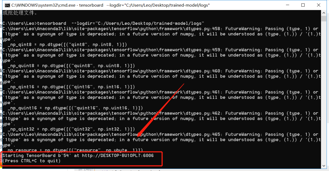
接着复制这个链接到浏览器打开:
本文电子版 后台回复 TF 获取