Python 代码实战：HOG 特征提取与 FDA 助力图像分类与投影可视化

该代码主要利用图像的方向梯度直方图（HOG）特征，基于线性判别分析（LDA/FDA 思路）实现功能。先是组织正、负样本数据及提取特征，接着计算类内、类间散度矩阵求投影向量，用于投影、分类，最后算出准确率并可视化投影结果。

代码如下：

import time
import cv2
import numpy as np
from matplotlib import pyplot as plt
from skimage.feature import hog

nDim = 144
nTrain = 40
nTot = 50
nTest = nTot - nTrain

# organizing data
posTrainData = np.zeros(shape=(nTrain, nDim))
for i in range(1, nTrain + 1):
    im = cv2.imread("E:/data/5/{}.jpg".format(i), 0)
    aFeat = hog(im, block_norm='L2', pixels_per_cell=(8, 8), cells_per_block=(2, 2))
    posTrainData[i - 1] = aFeat
negTrainData = np.zeros(shape=(nTrain, nDim))
for i in range(1, nTrain + 1):
    im = cv2.imread("E:/data/8/{}.jpg".format(i), 0)
    aFeat = hog(im, block_norm='L2', pixels_per_cell=(8, 8), cells_per_block=(2, 2))
    negTrainData[i - 1] = aFeat
testData = np.zeros(shape=(nTest * 2, nDim))
for i in range(nTrain + 1, nTot + 1):
    im = cv2.imread("E:/data/5/{}.jpg".format(i), 0)
    aFeat = hog(im, block_norm='L2', pixels_per_cell=(8, 8), cells_per_block=(2, 2))
    testData[i - nTrain - 1] = aFeat
for i in range(nTrain + 1, nTot + 1):
    im = cv2.imread("E:/data/8/{}.jpg".format(i), 0)
    aFeat = hog(im, block_norm='L2', pixels_per_cell=(8, 8), cells_per_block=(2, 2))
    testData[nTest + i - nTrain - 1] = aFeat

# organize test label for evaluation
testLabel = np.vstack((np.zeros(shape=(nTest, 1)), np.ones(shape=(nTest, 1))))

# FDA calculation
m1 = posTrainData.mean(axis=0).reshape(-1, 1)
m2 = negTrainData.mean(axis=0).reshape(-1, 1)
sigma_pos = np.zeros((nDim, nDim))
for i in range(0, nTrain):
    a = posTrainData[i, :]
    tmp = (posTrainData[i, :].reshape(-1, 1) - m1)  # 转为列向量
    sigma_pos += np.matmul(tmp, tmp.T)
sigma_pos /= nTrain
sigma_neg = np.zeros((nDim, nDim))
for i in range(0, nTrain):
    tmp = (negTrainData[i, :].reshape(-1, 1) - m2)  # 转为列向量
    sigma_neg += np.matmul(tmp, tmp.T)
sigma_neg /= nTrain
sw = sigma_pos + sigma_neg  # 1 计算类内散度矩阵 sw

start = time.perf_counter()
sb = np.matmul((m1 - m2), (m1 - m2).T)  # 2 计算类间散度矩阵 sb
tmpMat = np.matmul(np.linalg.pinv(sw), sb)
lam, v = np.linalg.eig(tmpMat)
lam = lam.real
v = v.real
# 取最大的特征根对应的特征向量
aIdx = np.argsort(lam)[::-1][0]
omega = v[:, aIdx].reshape(-1, 1)
end = time.perf_counter()
print('time: {:.3f}.'.format(end - start))

# 快速求法（根据瑞利商性质，omega 是 (sw^{-1} * sb) 最大特征值对应的特征向量，可通过广义特征值问题求解）
start = time.perf_counter()
eig_vals, eig_vecs = np.linalg.eig(np.linalg.solve(sw, sb))  # 3 利用广义特征值求解得到特征值和特征向量
aIdx_fast = np.argmax(eig_vals)
omega1 = eig_vecs[:, aIdx_fast].reshape(-1, 1)
end = time.perf_counter()
print('time1: {:.3f}.'.format(end - start))

# omega = omega1 #4 验证两种解法的omega有没有区别
# omega = omega / np.linalg.norm(omega, ord=2) #5 验证omega是否归一化有没有影响


# projection
posProj = np.matmul(posTrainData, omega)
negProj = np.matmul(negTrainData, omega)

# classification
bias = -0.5 * (np.mean(posProj) + np.mean(negProj))
yPred = np.matmul(testData, omega) + bias
pLabel = np.array([0 if x > 0 else 1 for x in yPred]).reshape(-1, 1)
acc = np.mean(pLabel == testLabel)
print('The accuracy is: {:.3f}! \n'.format(acc))

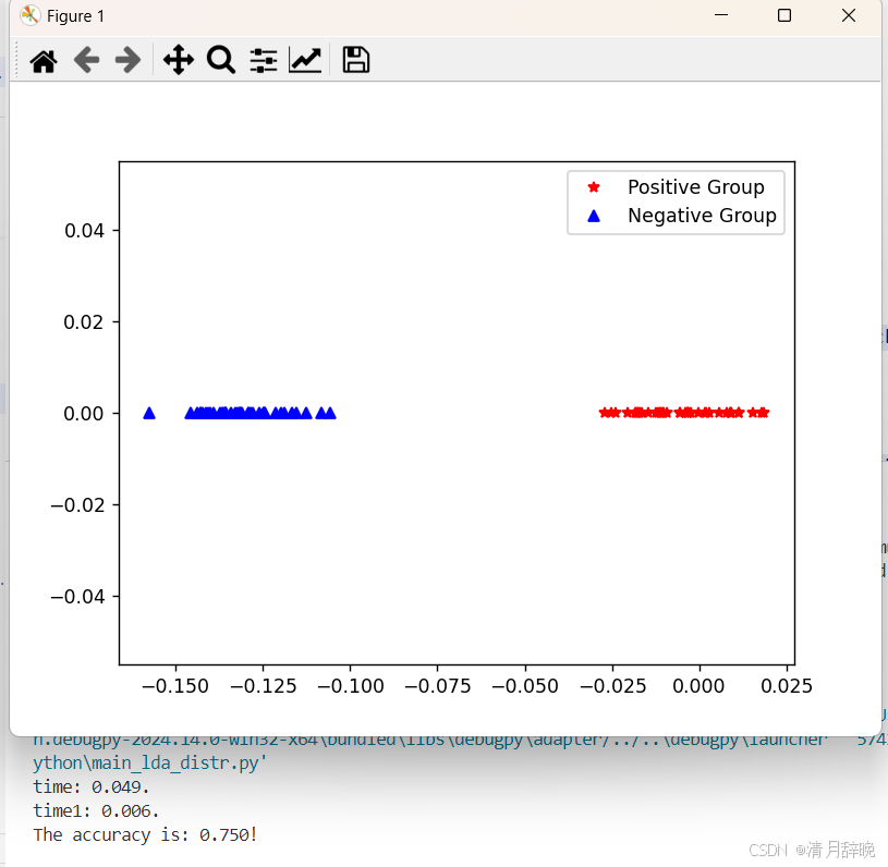
# visualize the projection
plt.figure()
plt.plot(posProj, np.zeros(nTrain), 'r*', label="Positive Group")  # Red asterisks
plt.plot(negProj, np.zeros(nTrain), 'b^', label="Negative Group")  # Blue triangles
plt.legend()
plt.show()

结果如下：