文章目录
一、准备工作
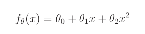
1. 以矩阵的形式来处理:

2. 参数更新表达式:
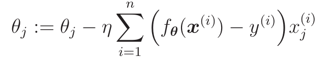

j=0时,把f转置之后与x0相乘,就与和的部分一样:
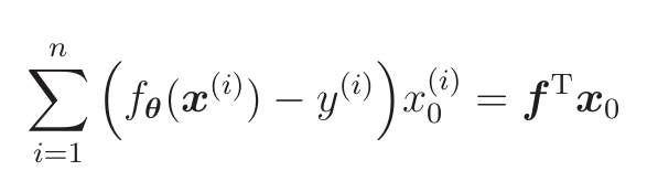
j=1,j=2也得到同样的结果,所以整个求和的计算可以写成:![]()
二、完整代码
import numpy as np
import matplotlib.pyplot as plt
# 读入训练数据
train = np.loadtxt('click.csv', delimiter=',', dtype='int', skiprows=1)
train_x = train[:,0]
train_y = train[:,1]
# 标准化
mu = train_x.mean()
sigma = train_x.std()
def standardize(x):
return (x - mu) / sigma
train_z = standardize(train_x)
# 参数初始化
theta = np.random.rand(3)
# 创建训练数据的矩阵
def to_matrix(x):
return np.vstack([np.ones(x.size), x, x ** 2]).T # 列堆叠为矩阵
X = to_matrix(train_z) # 设计矩阵示例:
# [[1, z1, z1^2],
# [1, z2, z2^2],
# ...]
# 预测函数
def f(x):
return np.dot(x, theta) # 矩阵乘法:X * theta
# 目标函数
def E(x, y):
return 0.5 * np.sum((y - f(x)) ** 2)
# 学习率
ETA = 1e-3
# 误差的差值
diff = 1
# 更新次数
count = 0
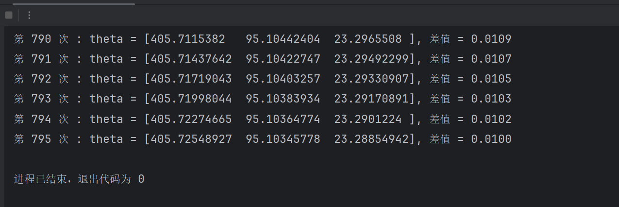
# 直到误差的差值小于 0.01 为止,重复参数更新
error = E(X, train_y)
while diff > 1e-2:
# 更新结果保存到临时变量
theta = theta - ETA * np.dot(f(X) - train_y, X)
# 计算与上一次误差的差值
current_error = E(X, train_y)
diff = error - current_error
error = current_error
# 输出日志
count += 1
log = '第 {} 次 : theta = {}, 差值 = {:.4f}'
print(log.format(count, theta, diff))
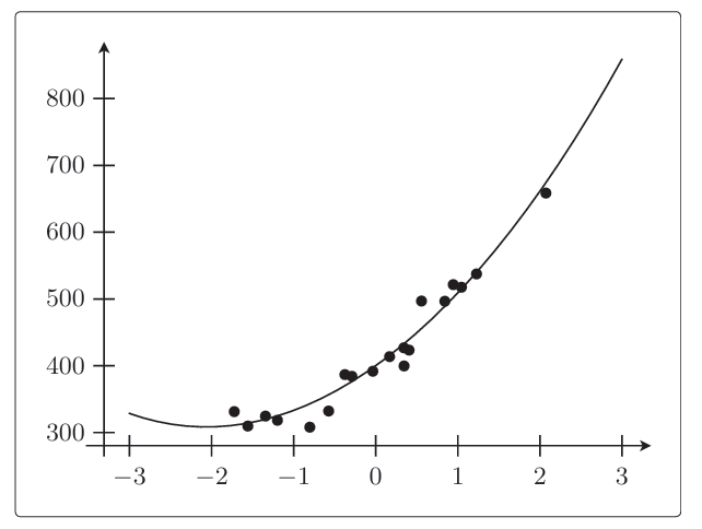
# 绘图确认
x = np.linspace(-3, 3, 100)
plt.plot(train_z, train_y, 'o')
plt.plot(x, f(to_matrix(x)))
plt.show()
三、实现效果
四、实现随机梯度下降
1. 参数更新表达式:

有了训练数据的矩阵X,把行的顺序随机地予以调整, 然后重复应用更新表达式就行了。
2. 代码修改部分:
# 重复学习
error = MSE(X, train_y)
while diff > 1e-2:
    # 使用随机梯度下降法更新参数
    p = np.random.permutation(X.shape[0])      # 为了调整训练数据的顺序,准备随机的序列
    for x, y in zip(X[p,:], train_y[p]):       # 随机取出训练数据,使用随机梯度下降法更新参数
        theta = theta - ETA * (f(x) - y) * x

    # 计算与上一次误差的差值
    current_error = MSE(X, train_y)
    diff = error - current_error
    error = current_error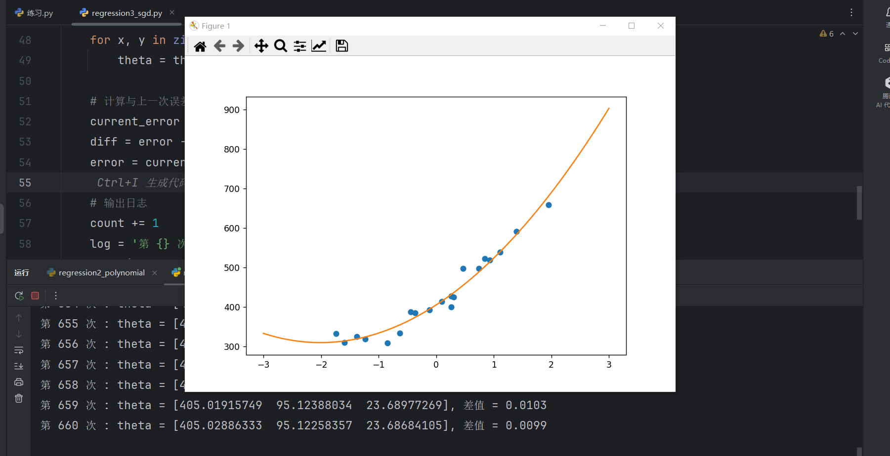
使用随机梯度下降后,计算次数减少,拟合的效果也不错。
五、拓展
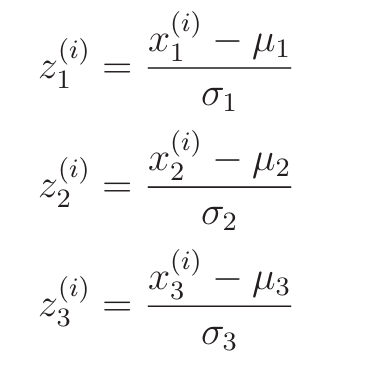
对于多重回归的实现,也可以像多项式回归时那样使用矩阵,要注意对多重回归的变量进行标准化时, 必须对每个参数都进行标准化。如果有变量x1、x2、x3,就要分别使用每个变量的平均值和标准差进行标准化。