正弦信号频谱分析实验
实验目标
【1】设定采样率fs,生成正弦波,频率为f0,量化比特数为Q,幅度为A,采集N点正弦波,用W窗对采样帧加窗,然后进行N点的FFT分析,观察对数尺度下的幅度谱S。
参考实验:
频率f0=20.0E3,量化比特数Q=12,幅度A=10;N=512,W窗为kaiser窗
%///////////////////////////////////////////////////////////
% DFT analyse of sampled sine signal
%///////////////////////////////////////////////////////////
close all;
clear;
clc;
% generate 2 sampled sine signals with different frequency(生成2个不同频率的采样正弦信号)
freq_x1 = 20.0E3 ; % frequency of signal x1
amp_x1 = 10 ; % amptitude of signal x1
freq_x2 = 30.0E3 ; % frequency of signal x2
amp_x2 = 10 ; % amptitude of signal x2
data_len = 512 ; % signal data length
fs = 512E3 ; % sample rate(采样率)
quant_bits = 12 ; % signal quant bits(信号量化比特数)
kaiser_beta = 8 ; % beta of kaiser win
idx_n = [0:data_len-1]; % n index
idx_n = idx_n .' ; % we need column vector(列向量)
idx_t = idx_n/fs ; % time index
idx_phase_x1 = 2*pi*idx_n*freq_x1/fs; % x1 phase index(x1相位指数)
idx_phase_x2 = 2*pi*idx_n*freq_x2/fs; % x2 phase index
x1 = amp_x1*sin(idx_phase_x1);
x2 = amp_x2*sin(idx_phase_x2);
% signal x is consisted of x1 and x2;
x = x1 + x2;
max_abs_x = max(abs(x)); % abs-求数值的绝对值与复数的幅值 % normalize x to (-1,1)
x = x / max_abs_x; % quant signal, the range is (-max_q, +max_q)
max_q = 2^(quant_bits-1);
x_quant = fix(x * max_q); % plot them, use time label
figure;
set(gca,'fontsize',16); % get window function data(获取窗口函数数据)(set-设置对象属性)
win = kaiser(data_len, kaiser_beta); % windowing the data
win_x = win .* x;
win_x_quant = win .* x_quant;
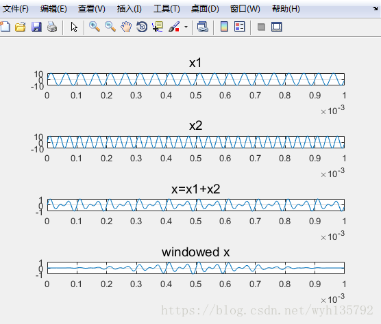
h_t1 = subplot(4,1,1);plot(idx_t, x1 );grid on;
h_t2 = subplot(4,1,2);plot(idx_t, x2 );grid on;
h_t3 = subplot(4,1,3);plot(idx_t, x );grid on;
h_t4 = subplot(4,1,4);plot(idx_t, win_x);grid on;
title(h_t1, 'x1' , 'fontsize', 14);
title(h_t2, 'x2' , 'fontsize', 14);
title(h_t3, 'x=x1+x2' , 'fontsize', 14);
title(h_t4, 'windowed x', 'fontsize', 14);
% perform fft(fft变换)
x_q_fft = fft(win_x_quant) ; % get frequency index(指数)
idx_freq = -fs/2 + idx_n .* (fs / data_len);
% shift zero frequency to the data center(将0频移动到数据中心位置)
x_q_fft = fftshift(x_q_fft);
% map to amptitude dB scale
x_q_fft_abs = abs(x_q_fft);
x_q_fft_abs_dB = 20*log10(x_q_fft_abs + 1E-8);
% normalize the spectrum from 0 dB;(从0db开始归一化频谱)
max_dB = max(x_q_fft_abs_dB);
norm_spectrum = x_q_fft_abs_dB - max_dB;
figure; plot(idx_freq, norm_spectrum);grid on;
title('Normlized Spectrum ', 'fontsize', 14);实验结果如下:
频谱S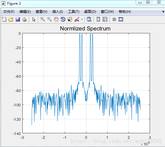
【2】对以上过程的参数, fs, f0, Q, A, N, W 进行修改,观察S的变化