Datawhale17期-task2

import pandas as pd
import numpy as np
import matplotlib.pyplot as plt
import seaborn as sns
import datetime
import warnings
warnings.filterwarnings('ignore')

#读取文件   如果文件太大，可在read_csv中设置参数读取多少行
data_train = pd.read_csv("./dataset/train.csv")   

data_test_a = pd.read_csv("./dataset/testA.csv")

#查看数据样本数和数据维度
print(data_train.shape)
print(data_test_a.shape)

(800000, 47)
(200000, 48)

#查看数据列
print(data_train.columns)

Index(['id', 'loanAmnt', 'term', 'interestRate', 'installment', 'grade',
       'subGrade', 'employmentTitle', 'employmentLength', 'homeOwnership',
       'annualIncome', 'verificationStatus', 'issueDate', 'isDefault',
       'purpose', 'postCode', 'regionCode', 'dti', 'delinquency_2years',
       'ficoRangeLow', 'ficoRangeHigh', 'openAcc', 'pubRec',
       'pubRecBankruptcies', 'revolBal', 'revolUtil', 'totalAcc',
       'initialListStatus', 'applicationType', 'earliesCreditLine', 'title',
       'policyCode', 'n0', 'n1', 'n2', 'n2.1', 'n4', 'n5', 'n6', 'n7', 'n8',
       'n9', 'n10', 'n11', 'n12', 'n13', 'n14'],
      dtype='object')

#通过info熟悉数据类型
data_train.info()

<class 'pandas.core.frame.DataFrame'>
RangeIndex: 800000 entries, 0 to 799999
Data columns (total 47 columns):
id                    800000 non-null int64
loanAmnt              800000 non-null float64
term                  800000 non-null int64
interestRate          800000 non-null float64
installment           800000 non-null float64
grade                 800000 non-null object
subGrade              800000 non-null object
employmentTitle       799999 non-null float64
employmentLength      753201 non-null object
homeOwnership         800000 non-null int64
annualIncome          800000 non-null float64
verificationStatus    800000 non-null int64
issueDate             800000 non-null object
isDefault             800000 non-null int64
purpose               800000 non-null int64
postCode              799999 non-null float64
regionCode            800000 non-null int64
dti                   799761 non-null float64
delinquency_2years    800000 non-null float64
ficoRangeLow          800000 non-null float64
ficoRangeHigh         800000 non-null float64
openAcc               800000 non-null float64
pubRec                800000 non-null float64
pubRecBankruptcies    799595 non-null float64
revolBal              800000 non-null float64
revolUtil             799469 non-null float64
totalAcc              800000 non-null float64
initialListStatus     800000 non-null int64
applicationType       800000 non-null int64
earliesCreditLine     800000 non-null object
title                 799999 non-null float64
policyCode            800000 non-null float64
n0                    759730 non-null float64
n1                    759730 non-null float64
n2                    759730 non-null float64
n2.1                  759730 non-null float64
n4                    766761 non-null float64
n5                    759730 non-null float64
n6                    759730 non-null float64
n7                    759730 non-null float64
n8                    759729 non-null float64
n9                    759730 non-null float64
n10                   766761 non-null float64
n11                   730248 non-null float64
n12                   759730 non-null float64
n13                   759730 non-null float64
n14                   759730 non-null float64
dtypes: float64(33), int64(9), object(5)
memory usage: 286.9+ MB

data_train.describe()   #百分数代表此列中位于数据位于 a%位置的数

	id	loanAmnt	term	interestRate	installment	employmentTitle	homeOwnership	annualIncome	verificationStatus	isDefault	...	n5	n6	n7	n8	n9	n10	n11	n12	n13	n14
count	800000.000000	800000.000000	800000.000000	800000.000000	800000.000000	799999.000000	800000.000000	8.000000e+05	800000.000000	800000.000000	...	759730.000000	759730.000000	759730.000000	759729.000000	759730.000000	766761.000000	730248.000000	759730.000000	759730.000000	759730.000000
mean	399999.500000	14416.818875	3.482745	13.238391	437.947723	72005.351714	0.614213	7.613391e+04	1.009683	0.199513	...	8.107937	8.575994	8.282953	14.622488	5.592345	11.643896	0.000815	0.003384	0.089366	2.178606
std	230940.252015	8716.086178	0.855832	4.765757	261.460393	106585.640204	0.675749	6.894751e+04	0.782716	0.399634	...	4.799210	7.400536	4.561689	8.124610	3.216184	5.484104	0.030075	0.062041	0.509069	1.844377
min	0.000000	500.000000	3.000000	5.310000	15.690000	0.000000	0.000000	0.000000e+00	0.000000	0.000000	...	0.000000	0.000000	0.000000	1.000000	0.000000	0.000000	0.000000	0.000000	0.000000	0.000000
25%	199999.750000	8000.000000	3.000000	9.750000	248.450000	427.000000	0.000000	4.560000e+04	0.000000	0.000000	...	5.000000	4.000000	5.000000	9.000000	3.000000	8.000000	0.000000	0.000000	0.000000	1.000000
50%	399999.500000	12000.000000	3.000000	12.740000	375.135000	7755.000000	1.000000	6.500000e+04	1.000000	0.000000	...	7.000000	7.000000	7.000000	13.000000	5.000000	11.000000	0.000000	0.000000	0.000000	2.000000
75%	599999.250000	20000.000000	3.000000	15.990000	580.710000	117663.500000	1.000000	9.000000e+04	2.000000	0.000000	...	11.000000	11.000000	10.000000	19.000000	7.000000	14.000000	0.000000	0.000000	0.000000	3.000000
max	799999.000000	40000.000000	5.000000	30.990000	1715.420000	378351.000000	5.000000	1.099920e+07	2.000000	1.000000	...	70.000000	132.000000	79.000000	128.000000	45.000000	82.000000	4.000000	4.000000	39.000000	30.000000

8 rows × 42 columns

#缺失值处理，   查看数据缺失值   isnull用法（https://pandas.pydata.org/docs/reference/api/pandas.DataFrame.isnull.html#pandas.DataFrame.isnull）  
print(f'There are {data_train.isnull().any().sum()} columns in train dataset with missing values.')

There are 22 columns in train dataset with missing values.

##查看缺失特征中缺失率大于50%的特征
have_null_fea_dict = (data_train.isnull().sum() / len(data_train)).to_dict()
fea_null_moreThanHalf = {
    
    }
for k ,v  in have_null_fea_dict.items():
    if v > 0.5:
        fea_null_moreThanHalf[k] = v
print(fea_null_moreThanHalf)

{}

# 具体查看缺失特征和缺失率
missing = data_train.isnull().sum() / len(data_train)
missing = missing[missing > 0]
missing.sort_values(inplace=True)
missing.plot.bar()

<matplotlib.axes._subplots.AxesSubplot at 0x2c80fdaa518>

#查看数据集中，特征属性只有一值的特征
one_value_fea = [col for col in data_train.columns if data_train[col].nunique() <= 1]
one_value_fea_test = [col for col in data_test_a.columns if data_test_a[col].nunique() <= 1]
print(one_value_fea)
print(one_value_fea_test)

['policyCode']
['policyCode']

总结

47列中有22列列缺少数据，很符合真实数据的情况。policyCode具有一个唯一值（等价于全部缺失）。有很多连续变量和一些分类变量

查看数据的数值类型、对象类型。类别特征，数值特征（连续性、离散型）

numerical_fea = list(data_train.select_dtypes(exclude=['object']).columns)   #select_dtypes选择特定类型的列，exclude表示排除的列的类型，object表示字符串类的
category_fea = list(filter(lambda x:x not in numerical_fea, list(data_train.columns)))
print(numerical_fea)

['id', 'loanAmnt', 'term', 'interestRate', 'installment', 'employmentTitle', 'homeOwnership', 'annualIncome', 'verificationStatus', 'isDefault', 'purpose', 'postCode', 'regionCode', 'dti', 'delinquency_2years', 'ficoRangeLow', 'ficoRangeHigh', 'openAcc', 'pubRec', 'pubRecBankruptcies', 'revolBal', 'revolUtil', 'totalAcc', 'initialListStatus', 'applicationType', 'title', 'policyCode', 'n0', 'n1', 'n2', 'n2.1', 'n4', 'n5', 'n6', 'n7', 'n8', 'n9', 'n10', 'n11', 'n12', 'n13', 'n14']

print(category_fea)

['grade', 'subGrade', 'employmentLength', 'issueDate', 'earliesCreditLine']

#查看grade列的值是否为对象类型
data_train.grade

0         E
1         D
2         D
3         A
4         C
5         A
6         A
7         C
8         C
9         B
10        B
11        E
12        D
13        B
14        A
15        B
16        D
17        B
18        E
19        E
20        C
21        C
22        D
23        C
24        A
25        A
26        B
27        C
28        A
29        C
         ..
799970    B
799971    A
799972    G
799973    D
799974    B
799975    E
799976    C
799977    C
799978    B
799979    C
799980    C
799981    C
799982    B
799983    B
799984    C
799985    D
799986    C
799987    B
799988    C
799989    D
799990    C
799991    B
799992    C
799993    A
799994    E
799995    C
799996    A
799997    C
799998    A
799999    B
Name: grade, Length: 800000, dtype: object

对于数值型变量，进行连续型和离散型变量划分

def get_numerical_serial_fea(data, feas):
    numerical_serial_fea = []
    numerical_noserial_fea = []
    for fea in feas:
        temp = data[fea].nunique()   #nunique统计某列不同类型的特征值有几种
        if temp <= 10:
            numerical_noserial_fea.append(fea)   #特征值的种类小于等于10，属于离散型变量
            continue
        numerical_serial_fea.append(fea)
    return numerical_serial_fea, numerical_noserial_fea

numerical_serial_fea, numerical_noserial_fea = get_numerical_serial_fea(data_train, numerical_fea)

numerical_serial_fea

['id',
 'loanAmnt',
 'interestRate',
 'installment',
 'employmentTitle',
 'annualIncome',
 'purpose',
 'postCode',
 'regionCode',
 'dti',
 'delinquency_2years',
 'ficoRangeLow',
 'ficoRangeHigh',
 'openAcc',
 'pubRec',
 'pubRecBankruptcies',
 'revolBal',
 'revolUtil',
 'totalAcc',
 'title',
 'n0',
 'n1',
 'n2',
 'n2.1',
 'n4',
 'n5',
 'n6',
 'n7',
 'n8',
 'n9',
 'n10',
 'n13',
 'n14']

numerical_noserial_fea

['term',
 'homeOwnership',
 'verificationStatus',
 'isDefault',
 'initialListStatus',
 'applicationType',
 'policyCode',
 'n11',
 'n12']

数值类别型变量分析
value_counts()用法

data_train['term'].value_counts()  #离散型变量   value_counts统计每一类特征值的个数

3    606902
5    193098
Name: term, dtype: int64

data_train['homeOwnership'].value_counts()

0    395732
1    317660
2     86309
3       185
5        81
4        33
Name: homeOwnership, dtype: int64

data_train['verificationStatus'].value_counts()

1    309810
2    248968
0    241222
Name: verificationStatus, dtype: int64

data_train["initialListStatus"].value_counts()

0    466438
1    333562
Name: initialListStatus, dtype: int64

data_train['applicationType'].value_counts()

0    784586
1     15414
Name: applicationType, dtype: int64

data_train["policyCode"].value_counts()  #离散型变量，全是一个值，无用

1.0    800000
Name: policyCode, dtype: int64

data_train['n11'].value_counts()  #离散型变量，相差悬殊，是否使用需根据后续分析

0.0    729682
1.0       540
2.0        24
4.0         1
3.0         1
Name: n11, dtype: int64

data_train['n12'].value_counts()#离散型变量， 相差悬殊， 是否使用根据后续分析

0.0    757315
1.0      2281
2.0       115
3.0        16
4.0         3
Name: n12, dtype: int64

数值连续型变量分析

f = pd.melt(data_train, value_vars=numerical_serial_fea)
g = sns.FacetGrid(f, col = "variable", col_wrap = 2, sharex = False, sharey = False)
g = g.map(sns.distplot, "value")

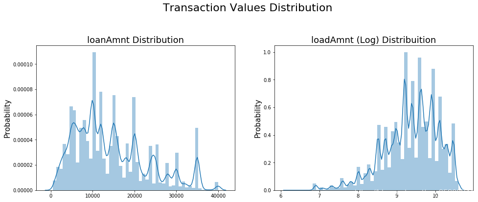
1. 通过上述可视化图可直观观察到数据是否服从正态化分布，不服从正太分布的变量，可对其进行求log后在观察
2. 正态化原因：某些模型对于正态化或非正态化数据的收敛速度不一样，有的快有的慢，一些模型要求数据正太（如GMM、KNN），保证数据不要过偏态即可，过于偏态可能会影响模型预测结果。

#成交金额（loadAmnt）价值分布
plt.figure(figsize = (16, 12))
plt.suptitle("Transaction Values Distribution", fontsize = 22)
plt.subplot(221)
sub_plot_1 = sns.distplot(data_train['loanAmnt'])
sub_plot_1.set_title("loanAmnt Distribution", fontsize = 18)
sub_plot_1.set_xlabel("")
sub_plot_1.set_ylabel("Probability", fontsize = 15)

plt.subplot(222)
sub_plot_2 = sns.distplot(np.log(data_train['loanAmnt']))
sub_plot_2.set_title("loadAmnt (Log) Distribuition", fontsize = 18)
sub_plot_2.set_xlabel("")
sub_plot_2.set_ylabel("Probability", fontsize = 15)

Text(0,0.5,'Probability')

非数值类别型变量分析

category_fea

['grade', 'subGrade', 'employmentLength', 'issueDate', 'earliesCreditLine']

data_train['grade'].value_counts()

B    233690
C    227118
A    139661
D    119453
E     55661
F     19053
G      5364
Name: grade, dtype: int64

data_train["subGrade"].value_counts()

C1    50763
B4    49516
B5    48965
B3    48600
C2    47068
C3    44751
C4    44272
B2    44227
B1    42382
C5    40264
A5    38045
A4    30928
D1    30538
D2    26528
A1    25909
D3    23410
A3    22655
A2    22124
D4    21139
D5    17838
E1    14064
E2    12746
E3    10925
E4     9273
E5     8653
F1     5925
F2     4340
F3     3577
F4     2859
F5     2352
G1     1759
G2     1231
G3      978
G4      751
G5      645
Name: subGrade, dtype: int64

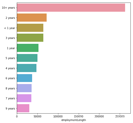
data_train["employmentLength"].value_counts()

10+ years    262753
2 years       72358
< 1 year      64237
3 years       64152
1 year        52489
5 years       50102
4 years       47985
6 years       37254
8 years       36192
7 years       35407
9 years       30272
Name: employmentLength, dtype: int64

data_train['issueDate'].value_counts()

2016-03-01    29066
2015-10-01    25525
2015-07-01    24496
2015-12-01    23245
2014-10-01    21461
2016-02-01    20571
2015-11-01    19453
2015-01-01    19254
2015-04-01    18929
2015-08-01    18750
2015-05-01    17119
2016-01-01    16792
2014-07-01    16355
2015-06-01    15236
2015-09-01    14950
2016-04-01    14248
2014-11-01    13793
2015-03-01    13549
2016-08-01    13301
2015-02-01    12881
2016-07-01    12835
2016-06-01    12270
2016-12-01    11562
2016-10-01    11245
2016-11-01    11172
2014-05-01    10886
2014-04-01    10830
2016-05-01    10680
2014-08-01    10648
2016-09-01    10165
              ...  
2010-01-01      355
2009-10-01      305
2009-09-01      270
2009-08-01      231
2009-07-01      223
2009-06-01      191
2009-05-01      190
2009-04-01      166
2009-03-01      162
2009-02-01      160
2009-01-01      145
2008-12-01      134
2008-03-01      130
2008-11-01      113
2008-02-01      105
2008-04-01       92
2008-01-01       91
2008-10-01       62
2007-12-01       55
2008-07-01       52
2008-08-01       38
2008-05-01       38
2008-06-01       33
2007-10-01       26
2007-11-01       24
2007-08-01       23
2007-07-01       21
2008-09-01       19
2007-09-01        7
2007-06-01        1
Name: issueDate, Length: 139, dtype: int64

data_train["earliesCreditLine"].value_counts()

Aug-2001    5567
Sep-2003    5403
Aug-2002    5403
Oct-2001    5258
Aug-2000    5246
Sep-2004    5219
Sep-2002    5170
Aug-2003    5116
Oct-2002    5034
Oct-2000    5034
Oct-2003    4969
Aug-2004    4904
Nov-2000    4798
Sep-2001    4787
Sep-2000    4780
Nov-1999    4773
Oct-1999    4678
Oct-2004    4647
Sep-2005    4608
Jul-2003    4586
Nov-2001    4514
Aug-2005    4494
Jul-2001    4480
Aug-1999    4446
Sep-1999    4441
Dec-2001    4379
Jul-2002    4342
Aug-2006    4283
Mar-2001    4268
May-2001    4223
            ... 
Sep-1961       2
Jul-1961       2
Oct-1958       2
Nov-1962       2
Feb-1959       2
Aug-1950       2
Feb-1961       2
May-1957       1
Oct-1957       1
Feb-1960       1
Aug-1955       1
Sep-1953       1
Dec-1951       1
May-1960       1
Nov-1953       1
Dec-1960       1
Jul-1955       1
Mar-1958       1
Aug-1946       1
Mar-1957       1
Aug-1958       1
Nov-1954       1
Sep-1957       1
Mar-1962       1
Jun-1958       1
Jan-1944       1
Oct-1954       1
Jan-1946       1
Apr-1958       1
Oct-2015       1
Name: earliesCreditLine, Length: 720, dtype: int64

data_train["isDefault"].value_counts()

0    640390
1    159610
Name: isDefault, dtype: int64

单一变量分布可视化

plt.figure(figsize = (8,8))
sns.barplot(data_train["employmentLength"].value_counts(dropna=False)[:20], data_train["employmentLength"].value_counts(dropna = False).keys()[:20])
plt.show()