文章目录
1. 频域滤波
% https://ccrma.stanford.edu/~jos/parshl/Overlap_Add_Synthesis.html
function overlap_add_synthesis
close all;
infile = 'P501_C_chinese_f1_FB_48k.wav';
infile = 'P501_C_chinese_m1_FB_48k.wav';
outfile = regexprep(infile, '\.wav', '_20200527_new.wav');
[data, fs] = audioread(infile); % 384000, 48k
%%
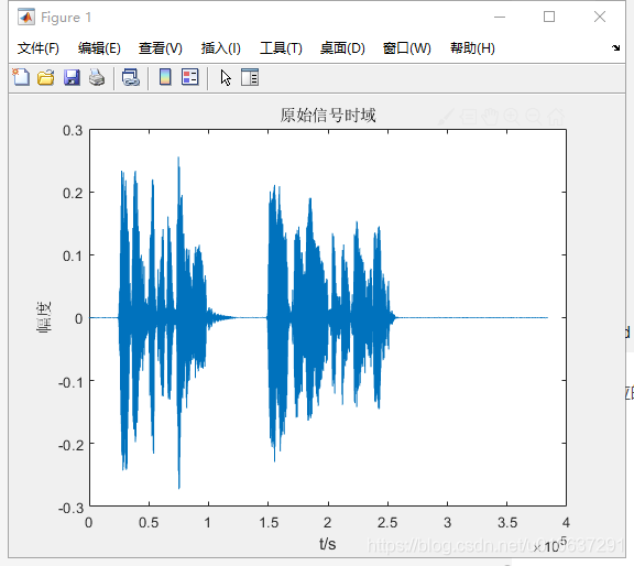
figure;
plot(data);
title('原始信号时域');
xlabel('t/s');
ylabel('幅度');
%%
frame_length = 1024;
frame_shift = 512;
frame_overlap = frame_length - frame_shift;
fftsize = 2^nextpow2(frame_length);
% hamming windows: sqrt would make the values larger, periodic
analysis_window = sqrt(hamming(frame_length, 'periodic'));
% analysis_window = ones(frame_length, 1); square windows
synthesis_window = analysis_window;
% 1024 * 749 (frame_length * num_frames)
x = buffer(data, frame_length, frame_overlap, 'nodelay'); % 'nodelay' means start from zero, withour padding
% Analysis windowing: (1024, 749) * (1024,1) could be multiplied by .*
x_anawin = x.*repmat(analysis_window(:), [1, size(x, 2)]);
% To frequency-domain
X = fft(x_anawin, fftsize); % default: fft(x_anawin, fftsize, 1);
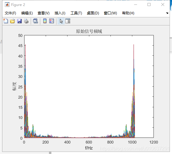
figure;
f = linspace(-24000, 24000, 1024);
plot(abs(X));
title('原始信号频域');
xlabel('f/Hz');
ylabel('幅度');
%%
% Modify the spectrum X here
% generate filter, i.e., (1024, 1)
x_f=[0, 1000, 2000, 3500, 24000];
y_f=[1, 0.98, 0.7, 0.55, 0.1];
% 1 means DC offset, X(k) should equal X(1026-k), thus X(513) is the
% center, X(512) = X(514), X(2) = X(1024), X(1) = DC offset.
xx=1:48000/1024:48000/1024*513;
fil=interp1(x_f,y_f,xx,'cubic');
% [513, 1026] 513 points, while X(513) and X(last) should be removed,
% since X(513) is contained in fil, X(last) is not used(X(0) has no synmetric point)
fil2=fliplr(fil);
fil2(1) = [];
fil2(512) = [];
fil = [fil fil2];
figure;
plot(fil);
X = X.* fil';
% X = X.* 0.2;
figure;
plot(f, abs(X));
% X(1:513,:) = X(1:513,:) * 0.2;
%%
% To time-domain
y = ifft(X);
% Synthesis windowing
y_synwin = y.* repmat(synthesis_window(:), [1, size(y, 2)]);
% Overlap-add
y_ola = y_synwin(:, 1);
for i = 2:size(y_synwin, 2)
y_ola(end+(1:frame_shift)) = zeros(frame_shift, 1);
y_ola(end+(-frame_length+1:0)) = y_ola(end+(-frame_length+1:0)) + y_synwin(:, i);
end
% Output
audiowrite(outfile, y_ola, fs);
end
对应的原始时域信号、频域信号、滤波器、滤波后的频域信号分别为:
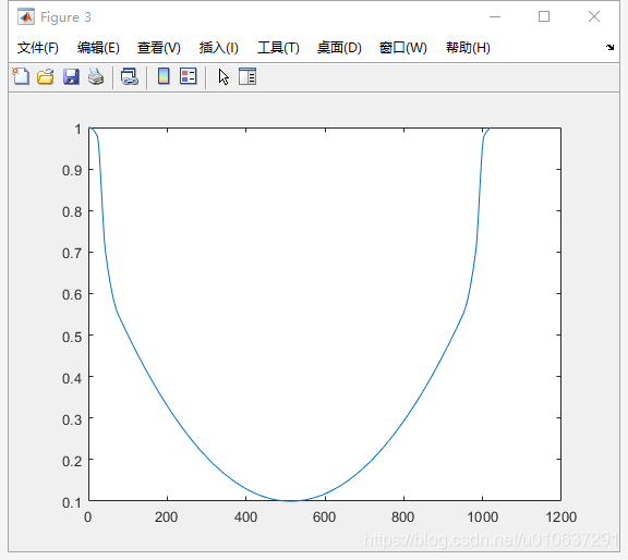
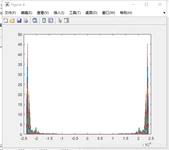
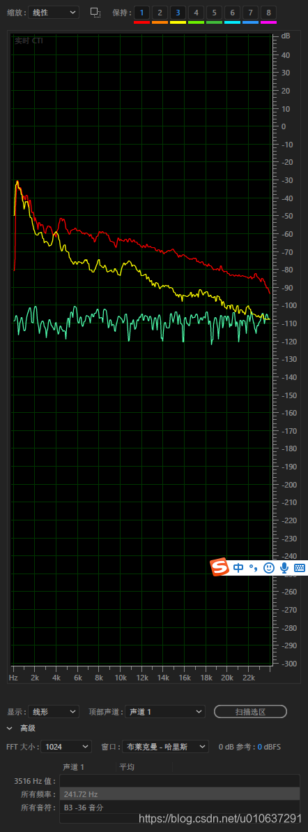
用adobe audition查看,即可看到频率被减小了,即实现了高通滤波器。
注:红色为原来的频率,黄色为滤波后的。
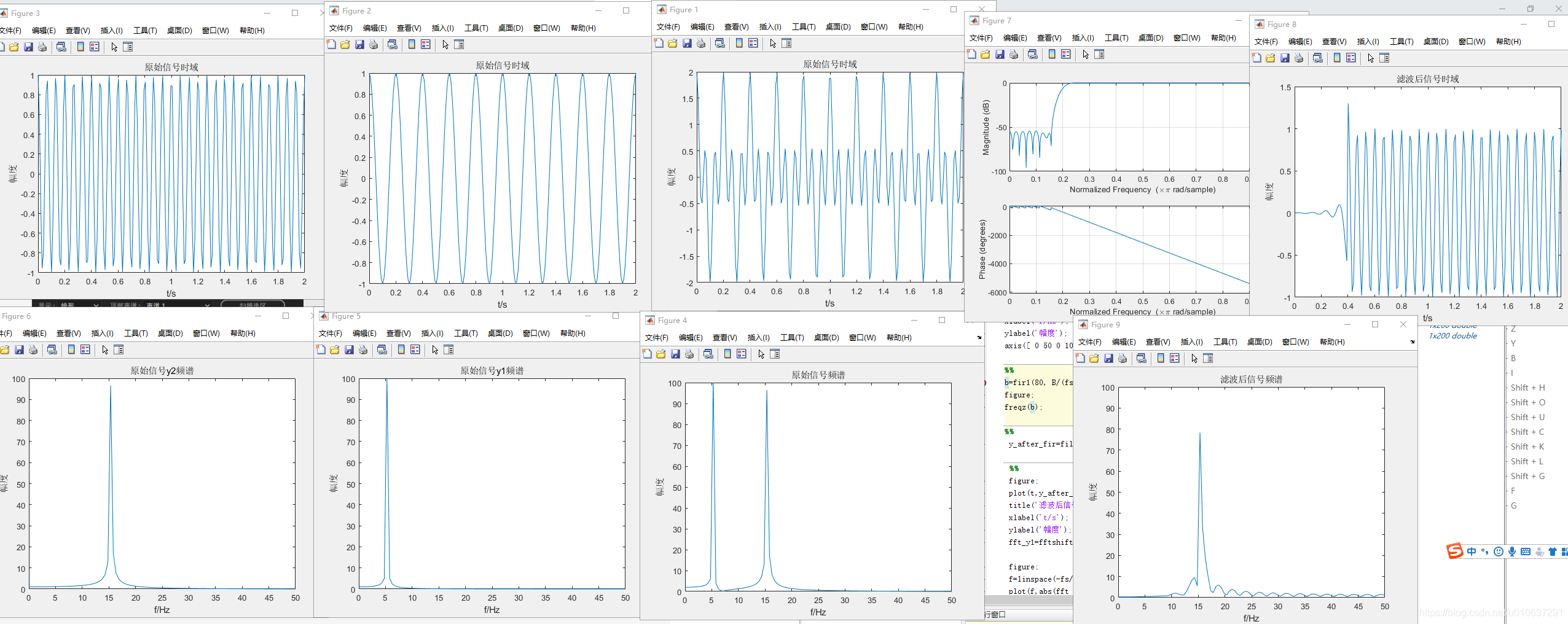
2. 时域滤波
f1=5;%第一个点频信号分量频率
f2=15;%第二个点频信号分量频率
fs=100;%采样率
T=2;%时宽
B=10;%FIR截止频率
n=round(T*fs);%采样点个数
t=linspace(0,T,n);
y1= cos(2*pi*f1*t);
y2=cos(2*pi*f2*t);
y=y1+y2;

%%
figure;
plot(t,y);
title('原始信号时域');
xlabel('t/s');
ylabel('幅度');

figure;
plot(t,y1);
title('原始信号时域');
xlabel('t/s');
ylabel('幅度');

figure;
plot(t,y2);
title('原始信号时域');
xlabel('t/s');
ylabel('幅度');

%%
figure;
fft_y=fftshift(fft(y));
f=linspace(-fs/2,fs/2,n);
plot(f,abs(fft_y));
title('原始信号频谱');
xlabel('f/Hz');
ylabel('幅度');
axis([ 0 50 0 100]);

figure;
fft_y=fftshift(fft(y1));
f=linspace(-fs/2,fs/2,n);
plot(f,abs(fft_y));
title('原始信号y1频谱');
xlabel('f/Hz');
ylabel('幅度');
axis([ 0 50 0 100]);

figure;
fft_y=fftshift(fft(y2));
f=linspace(-fs/2,fs/2,n);
plot(f,abs(fft_y));
title('原始信号y2频谱');
xlabel('f/Hz');
ylabel('幅度');
axis([ 0 50 0 100]);

%%
b=fir1(80, B/(fs/2),'high');                    %滤波产生指定带宽的噪声信号
figure;
freqz(b);

%%
 y_after_fir=filter(b,1,y);

 %%
 figure;
 plot(t,y_after_fir);
 title('滤波后信号时域');
 xlabel('t/s');
 ylabel('幅度');
 fft_y1=fftshift(fft(y_after_fir));

 figure;
 f=linspace(-fs/2,fs/2,n);
 plot(f,abs(fft_y1));
 title('滤波后信号频谱');
 xlabel('f/Hz');
 ylabel('幅度');
 axis([ 0 50 0 100]);
具体滤波结果如下图
Matlab 所用函数解释:
- regexprep(infile, ‘.wav’, ‘_20200527_new.wav’): 字符串替换,输入为原始字符串,需替换的字符串,及去替换的字符串; 输出为替换后的字符串。
- audioread(infile): 读取wav文件,输入为文件路径加文件名,输出为归一化后的sample值和采样率fs。
- plot(data):画图
- ^: 次方,如2的3次方为:2 ^ 3
- nextpow2(num): 比输入的数据大一点的2的幂次方,如输入15,则返回 4。注:只有nextpow2没有nextpow3及其它的。
- sqrt(num): 开方
- hamming(frame_length, ‘periodic’):汉明窗,HAMMING(N) returns the N-point symmetric Hamming window in a column vector. HAMMING(N,SFLAG) generates the N-point Hamming window using SFLAG window sampling. SFLAG may be either ‘symmetric’ or ‘periodic’. By default, a symmetric window is returned.
- buffer(data, frame_length, frame_overlap, ‘nodelay’):将数据存成矩阵,
- Y = BUFFER(X,N) partitions signal vector X into nonoverlapping data
% segments (frames) of length N. - Y = BUFFER(X,N,P) specifies an integer value P which controls the amount of overlap or underlap in the buffered data frames.
% - If P>0, there will be P samples of data from the end of one frame (column) that will be repeated at the start of the next data frame.
% - If P<0, the buffering operation will skip P samples of data after each frame, effectively skipping over data in X, and thus reducing the buffer “frame rate”.
% - If empty or omitted, P is assumed to be zero (no overlap or underlap). - Y = BUFFER(X,N,P,OPT) specifies an optional parameter OPT used in the case of overlap or underlap buffering.
% - If P>0 (overlap), OPT specifies an initial condition vector with length equal to the overlap, P. If empty or omitted, the initial condition is assumed to be zeros(P,1). Alternatively, OPT can be set to ‘nodelay’ which removes initial conditions from the output and starts buffering at the first data sample in X.
% - If P<0 (underlap), OPT specifies a scalar offset indicating the number of initial data samples in X to skip. The offset must be in the range [0, -P], where P<0. If empty or omitted, the offset is zero.
- Y = BUFFER(X,N) partitions signal vector X into nonoverlapping data