MATLAB信号处理之连续时间系统的时域分析

1、零状态响应
题目如下

我们用lsim(sys,f,t)来求解零状态响应，关于此函数用法看下图

代码如下

ts=0;te=5;dt=0.01;
sys=tf([2,-4],[1 5 4]);   %得到LTI系统模型，其实就是所要求解的微分方程的各项系数
t=ts:dt:te;
f=heaviside(t);           %设定激励为阶跃信号
yzs=lsim(sys,f,t);        %求解零状态响应
plot(t,yzs)
grid on
xlabel('t');
ylabel('yzs(t)');
title('零状态响应曲线')

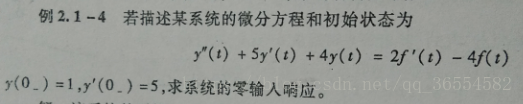
2、零输入响应
题目如下

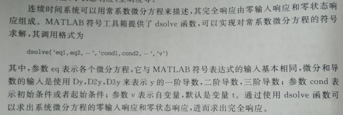
我们用dsolve(‘eq1,eq2,…’,’cond1,cond2,…’,’v’)函数来求解，关于此函数用法看下图

代码如下

eq='D2y+5*Dy+4*y=0';      %求解零输入响应时，激励应该令其为0
cond='y(0)=1,Dy(0)=5';    %初始条件
yzi=dsolve(eq,cond)

结果如下

yzi =

3*exp(-t) - 2*exp(-4*t)

3、冲激响应和阶跃响应
如果激励是冲激函数或者阶跃函数，我们除了用上面提到的两个函数（lsim(),dsolve()）外，还可以利用专门求解冲激响应和阶跃响应的函数，冲激响应h=impulse(sys,t)，阶跃响应g=step(sys,t)
代码如下

t=0:0.002:4;
sys=tf([1,32],[1,4,64]);      %LTI系统
h=impulse(sys,t);             %求解冲激响应
g=step(sys,t);                %求解阶跃响应
subplot(211)
plot(t,h)
grid on
xlabel('时间/s')
ylabel('h(t)');
title('冲激响应');
subplot(212)
plot(t,g)
grid on
xlabel('时间/s')
ylabel('g(t)');
title('阶跃响应')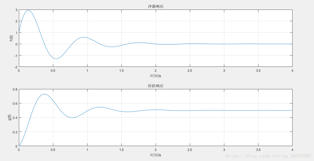

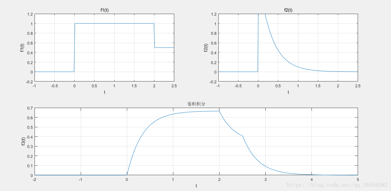
4、卷积
信号的卷积运算有符号算法和数值算法，此处采用数值计算法，需要调用MATLAB中的conv()函数来近似计算信号的卷积积分
例：用数值计算法求f1(t)=u(t)-0.5u(t-2)与f2(t)=2e^(-3t)u(t)的卷积积分，其中u(t)代表阶跃信号
代码如下

dt=0.01;
t=-1:dt:2.5;
f1=heaviside(t)-0.5*heaviside(t-2);
f2=2*exp(-3*t).*heaviside(t);
f=conv(f1,f2)*dt;
n=length(f);
tt=(0:n-1)*dt-2;
subplot(221)
plot(t,f1);
grid on
axis([-1,2.5,-0.2,1.2])
title('f1(t)');
xlabel('t')
ylabel('f1(t)');
subplot(222)
plot(t,f2);
grid on
axis([-1,2.5,-0.2,1.2])
title('f2(t)');
xlabel('t')
ylabel('f2(t)');
subplot(212)
plot(tt,f)
grid on
title('卷积积分')
xlabel('t')
ylabel('f3(t)')