信号是随时间和空间变化的某种物理量,它一般是时间变量t的函数。信号随时间变量t变化的函数曲线成为信号的波形。
本部分主要内容包括两块:
下面我将用Python+matplotlib的方式绘制动态图,从而直观地展示效果
1. 信号的时域变换
基本原理
信号在时域中的变换基本包括:
- 反转:信号的时域反转就是将信号f (t) 的波形以纵轴为对称轴为轴翻转180。其表达式为f(-t)。
- 时移:信号的时移就是将信号f(t)的波形沿时间轴t平移,但波形的形状不变。其表达式为f(t+t0),t0为正时左移,t0为负时右移。
- 展缩:信号的展缩就是将信号f(t)在时间轴上展缩或压缩,但纵轴上的值不变。其表达式为f(at),a>1时为压缩,a<1时为展宽。
下面来具体看一下这三种变换该如何实现,在这之前,先确定一个原来信号,下面的变换将在原信号的基础上进行:
import numpy as np
from matplotlib import pyplot as plt
from matplotlib import animation

# First set up the figure, the axis, and the plot element we want to animate
fig = plt.figure()
ax = plt.axes(xlim=(0, 4), ylim=(-4, 4))
line, = ax.plot([], [], lw=2)

# initialization function: plot the background of each frame
def init():
    line.set_data([], [])
    return line,

# animation function.  This is called sequentially
def animate(i):
    x = np.linspace(0, 4, 1000)
    y = np.sin(np.pi * (x - 0.01 * i))
    line.set_data(x,3*y)
    return line,

# call the animator.  blit=True means only re-draw the parts that have changed.
anim = animation.FuncAnimation(fig, animate, init_func=init,
                               frames=200, interval=20, blit=True)

plt.show()
效果如下所示:

这里我把几个比较重要的参数提一下:
- 横轴、纵轴的长度设置:
ax = plt.axes(xlim=(0, 4), ylim=(-4, 4)) - 准备横轴的数据,范围在0-4,生成1000个:
x = np.linspace(0, 4, 1000) - 准备纵轴的数据,求出对应横轴的sin函数值:
y = np.sin(np.pi * (x - 0.01 * i)) - 导入数据:
line.set_data(x, 3*y)
静态图如下:

为了更好地展示,这里最好是一个子图放两个信号做对比,所以我把代码优化了一下:
import numpy as np
from matplotlib import pyplot as plt
from matplotlib import animation


# First set up the figure, the axis, and the plot element we want to animate
fig = plt.figure()
ax1 = plt.axes(xlim=(0, 4), ylim=(-4, 4))
ax2 = plt.axes(xlim=(0, 4), ylim=(-4, 4))
line1, = ax1.plot([], [], lw=2, label='Original signal',color="green")
line2, = ax2.plot([], [], lw=2, label='Transformed signal',color="red")


# initialization function: plot the background of each frame
def init():
    line1.set_data([], [])
    line2.set_data([], [])
    return line1,line2

# animation function.  This is called sequentially
def animate(i):
    x = np.linspace(0, 4, 1000)
    y1 = np.cos(np.pi * (x - 0.01 * i)) #绿色
    y2 = -(np.cos(np.pi * (x - 0.01 * i))) #红色
    line1.set_data(x, y1)
    line2.set_data(x, y2)
    return line1,line2

# call the animator.  blit=True means only re-draw the parts that have changed.
anim = animation.FuncAnimation(fig, animate, init_func=init,
                               frames=200, interval=20, blit=True)

plt.legend()
plt.show()
加以说明一下:
- y1用于表示原信号,用绿色表现
- y2用于表示变换后的信号,用红色表现
下面主要展示的是animate方法里的代码,因为其余部分是不变的,实现以下信号变换,只需要修改几个参数即可,难度也不是很大
反转
反转是以纵轴为中心180度反转,即左右对折
很简单,在x前加个负号即可:
def animate(i):
    x = np.linspace(0, 4, 1000)
    y1 = np.cos(np.pi * (x - 0.01 * i)) #绿色
    y2 = np.sin(np.pi * ((-1) * x - 0.01 * i)) #红色
    line1.set_data(x, y1)
    line2.set_data(x, y2)
    return line1,line2
效果如下:

我们换成指数函数感受一下
这里要把子图的大小稍微改一下:
ax1 = plt.axes(xlim=(-25, 25), ylim=(-4, 100))
ax2 = plt.axes(xlim=(-25, 25), ylim=(-4, 100))
然后再来修改animate方法:
def animate(i):
    x = np.linspace(-4, 4, 1000)
    y1 = 2**x * i #绿色
    y2 = 2**(x*(-1)) * i  #红色
    line1.set_data(x, y1)
    line2.set_data(x, y2)
    return line1,line2

时移
这里我们给定一个值吧,将原信号左移1个单位 :
def animate(i):
    x = np.linspace(0, 4, 1000)
    y1 = np.cos(np.pi * (x - 0.01 * i)) #绿色
    y2 = np.cos(np.pi * (x - 0.01 * i) + 1) #红色
    line1.set_data(x, y1)
    line2.set_data(x, y2)
    return line1,line2

那么向右时移自然是减了,比如向右时移2个单位:
def animate(i):
    x = np.linspace(0, 4, 1000)
    y1 = np.cos(np.pi * (x - 0.01 * i)) #绿色
    y2 = np.cos(np.pi * (x - 0.01 * i) - 2) #红色
    line1.set_data(x, y1)
    line2.set_data(x, y2)
    return line1,line2
效果如下:

展缩
将原信号压缩成原来的一半:
def animate(i):
    x = np.linspace(0, 4, 1000)
    y1 = np.cos(np.pi * (x - 0.01 * i)) #绿色
    y2 = np.cos(np.pi * (x - 0.01 * i) * 2) #红色
    line1.set_data(x, y1)
    line2.set_data(x, y2)
    return line1,line2
用动图展示:

如果要展宽,只需要把值改成小于1的值即可,如展宽成原来的2倍:
def animate(i):
    x = np.linspace(0, 4, 1000)
    y1 = np.cos(np.pi * (x - 0.01 * i)) #绿色
    y2 = np.cos(np.pi * (x - 0.01 * i) * 1/2) #红色
    line1.set_data(x, y1)
    line2.set_data(x, y2)
    return line1,line2
效果如下:

2. 信号的基本运算
实验原理
信号在时域中的运算有相加、相减、相乘、数乘、微分、积分等。
-
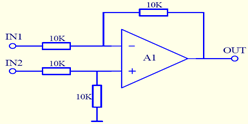
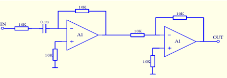
相加:信号在时域中相加时,其横坐标(时间轴)不变,仅是将横坐标所对应的值相加。两输入加法器:
加法器完成功能:OUT=IN1+IN2 -
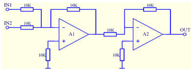
相减:信号在时域相减时,其横坐标不变,仅是将横坐标值对应的纵坐标值相减。减法器的电路如图所示:
减法器完成功能:OUT=IN2-IN1 -
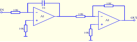
数乘:信号在时域倍乘时,其横坐标不变,仅是将横坐标值所对应的纵坐标值扩大n倍(n>1时扩大;0<n<1时减小)。倍乘器如图所示:
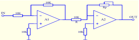
数乘器完成功能:OUT=(RP/R)*IN -
反相:信号在时域反相时,其横坐标不变,仅是将横坐标值所对应的纵坐标值乘负号。反相器电路如图所示:
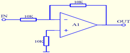
反相器完成功能:OUT=-IN -
微分:信号在时域微分即是对信号求一阶导数。微分器电路如图所示:
-
积分:信号在时域积分即将信号在(-∞,t)内求一次积分。积分器电路如图所示:
上面这些运算是通过电子元件来实现的,下面我们看一下如何用python实现相加、相减、相乘、数乘、微分、积分
相加
有了上面的基础,下面这几个基本运算其实也很好理解了,不就是多一个信号嘛:
def animate(i):
    x = np.linspace(0, 4, 1000)
    y1 = np.cos(np.pi * (x - 0.01 * i)) #绿色
    y21 = np.sin(np.pi * (x - 0.01 * i))
    y22 = np.sin(np.pi * (x - 0.01 * i))
    y2 = y21 + y22 #红色
    line1.set_data(x, y1)
    line2.set_data(x, y2)
    return line1,line2
两个标准的sin函数相加,得到的是:

这里不需要多说了吧?大家可以尝试改成其他的参数,试一下效果
相减
两个相同的信号相减会得到什么呢:
def animate(i):
    x = np.linspace(0, 4, 1000)
    y1 = np.cos(np.pi * (x - 0.01 * i)) #绿色
    y21 = np.sin(np.pi * (x - 0.01 * i))
    y22 = np.sin(np.pi * (x - 0.01 * i))
    y2 = y22 - y21 #红色
    line1.set_data(x, y1)
    line2.set_data(x, y2)
    return line1,line2
答案是一条直线:

那如果是这种情况,其中一个信号缩减为原来的一半:
def animate(i):
    x = np.linspace(0, 4, 1000)
    y1 = np.cos(np.pi * (x - 0.01 * i)) #绿色
    y21 = np.sin(np.pi * (x - 0.01 * i))
    y22 = np.sin(np.pi * (x - 0.01 * i) * 2)
    y2 = y22 - y21 #红色
    line1.set_data(x, y1)
    line2.set_data(x, y2)
    return line1,line2
效果如下:

当然,这里可以调的参数也有很多,这里就不一一举例了
数乘
这里的数乘不是两个信号相乘,对于某一信号在时域倍乘时,其横坐标不变,仅是将横坐标值所对应的纵坐标值扩大n倍
举个例子,原信号乘2:
def animate(i):
    x = np.linspace(0, 4, 1000)
    y1 = np.sin(np.pi * (x - 0.01 * i)) #绿色
    y2 = 2 * np.sin(np.pi * (x - 0.01 * i))
    line1.set_data(x, y1)
    line2.set_data(x, y2)
    return line1,line2
效果如下:

反相
信号的横坐标不变,仅是将横坐标值所对应的纵坐标值乘负号:
def animate(i):
    x = np.linspace(-4, 4, 1000)
    y1 = np.sin(np.pi * (x - 0.01 * i)) #绿色
    y2 = (-1) * np.sin(np.pi * (x - 0.01 * i)) #红色
    line1.set_data(x, y1)
    line2.set_data(x, y2)
    return line1,line2

这里要注意区分跟反转的区别,我们拿最简单的幂函数举例:
def animate(i):
    x = np.linspace(0, 4, 1000)
    y1 = x * i #绿色
    y2 = x * i * (-1) #红色
    line1.set_data(x, y1)
    line2.set_data(x, y2)
    return line1,line2
注意反相是上下对称的:

微分
我们知道sin(x)的微分是cos(x),所以这里直接改一下即可:
def animate(i):
    x = np.linspace(-4, 4, 1000)
    y1 = np.sin(np.pi * (x - 0.01 * i)) #绿色
    y2 = np.cos(np.pi * (x - 0.01 * i)) #红色
    line1.set_data(x, y1)
    line2.set_data(x, y2)
    return line1,line2
图像如下:

积分
同理,sin(x)在(-∞,t)的积分是-cos(t):

这样一来就好办了:
def animate(i):
    x = np.linspace(-4, 4, 1000)
    y1 = np.sin(np.pi * (x - 0.01 * i)) #绿色
    y2 = (-1) * np.cos(np.pi * (x - 0.01 * i)) #红色
    line1.set_data(x, y1)
    line2.set_data(x, y2)
    return line1,line2
如下图所示:
